穩健線性模型
[1]:
%matplotlib inline
[2]:
import matplotlib.pyplot as plt
import numpy as np
import statsmodels.api as sm
估計
載入資料
[3]:
data = sm.datasets.stackloss.load()
data.exog = sm.add_constant(data.exog)
具有(預設)中位數絕對偏差縮放的 Huber's T 範數
[4]:
huber_t = sm.RLM(data.endog, data.exog, M=sm.robust.norms.HuberT())
hub_results = huber_t.fit()
print(hub_results.params)
print(hub_results.bse)
print(
    hub_results.summary(
        yname="y", xname=["var_%d" % i for i in range(len(hub_results.params))]
    )
)
const       -41.026498
AIRFLOW       0.829384
WATERTEMP     0.926066
ACIDCONC     -0.127847
dtype: float64
const        9.791899
AIRFLOW      0.111005
WATERTEMP    0.302930
ACIDCONC     0.128650
dtype: float64
                    Robust linear Model Regression Results
==============================================================================
Dep. Variable:                      y   No. Observations:                   21
Model:                            RLM   Df Residuals:                       17
Method:                          IRLS   Df Model:                            3
Norm:                          HuberT
Scale Est.:                       mad
Cov Type:                          H1
Date:                Thu, 03 Oct 2024
Time:                        15:51:12
No. Iterations:                    19
==============================================================================
                 coef    std err          z      P>|z|      [0.025      0.975]
------------------------------------------------------------------------------
var_0        -41.0265      9.792     -4.190      0.000     -60.218     -21.835
var_1          0.8294      0.111      7.472      0.000       0.612       1.047
var_2          0.9261      0.303      3.057      0.002       0.332       1.520
var_3         -0.1278      0.129     -0.994      0.320      -0.380       0.124
==============================================================================

If the model instance has been used for another fit with different fit parameters, then the fit options might not be the correct ones anymore .
具有 ‘H2’ 共變異數矩陣的 Huber's T 範數
[5]:
hub_results2 = huber_t.fit(cov="H2")
print(hub_results2.params)
print(hub_results2.bse)
const       -41.026498
AIRFLOW       0.829384
WATERTEMP     0.926066
ACIDCONC     -0.127847
dtype: float64
const        9.089504
AIRFLOW      0.119460
WATERTEMP    0.322355
ACIDCONC     0.117963
dtype: float64
具有 Huber's Proposal 2 縮放和 ‘H3’ 共變異數矩陣的 Andrew's Wave 範數
[6]:
andrew_mod = sm.RLM(data.endog, data.exog, M=sm.robust.norms.AndrewWave())
andrew_results = andrew_mod.fit(scale_est=sm.robust.scale.HuberScale(), cov="H3")
print("Parameters: ", andrew_results.params)
Parameters:  const       -40.881796
AIRFLOW       0.792761
WATERTEMP     1.048576
ACIDCONC     -0.133609
dtype: float64
請參閱 help(sm.RLM.fit) 以取得更多選項,以及 module sm.robust.scale 以取得縮放選項
比較 OLS 和 RLM
具有離群值的人工資料
[7]:
nsample = 50
x1 = np.linspace(0, 20, nsample)
X = np.column_stack((x1, (x1 - 5) ** 2))
X = sm.add_constant(X)
sig = 0.3  # smaller error variance makes OLS<->RLM contrast bigger
beta = [5, 0.5, -0.0]
y_true2 = np.dot(X, beta)
y2 = y_true2 + sig * 1.0 * np.random.normal(size=nsample)
y2[[39, 41, 43, 45, 48]] -= 5  # add some outliers (10% of nsample)
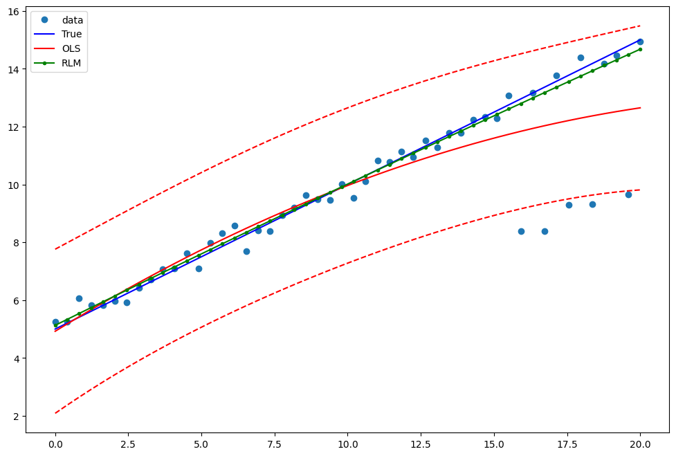
範例 1:具有線性真實值的二次函數
請注意,OLS 迴歸中的二次項將捕捉離群值效應。
[8]:
res = sm.OLS(y2, X).fit()
print(res.params)
print(res.bse)
print(res.predict())
[ 5.21792383  0.50415069 -0.01178124]
[0.43595638 0.06730578 0.00595552]
[ 4.92339275  5.17529253  5.42326685  5.66731574  5.90743917  6.14363717
  6.37590971  6.60425681  6.82867847  7.04917468  7.26574545  7.47839077
  7.68711064  7.89190507  8.09277405  8.28971759  8.48273568  8.67182833
  8.85699553  9.03823729  9.2155536   9.38894447  9.55840989  9.72394987
  9.8855644  10.04325348 10.19701712 10.34685531 10.49276806 10.63475536
 10.77281722 10.90695363 11.0371646  11.16345012 11.2858102  11.40424483
 11.51875401 11.62933775 11.73599605 11.8387289  11.9375363  12.03241826
 12.12337477 12.21040584 12.29351146 12.37269164 12.44794637 12.51927566
 12.5866795  12.65015789]
估計 RLM
[9]:
resrlm = sm.RLM(y2, X).fit()
print(resrlm.params)
print(resrlm.bse)
[ 5.15683122e+00  4.88535174e-01 -1.11256925e-03]
[0.12686184 0.01958576 0.00173304]
繪製圖表以比較 OLS 估計值與穩健估計值
[10]:
fig = plt.figure(figsize=(12, 8))
ax = fig.add_subplot(111)
ax.plot(x1, y2, "o", label="data")
ax.plot(x1, y_true2, "b-", label="True")
pred_ols = res.get_prediction()
iv_l = pred_ols.summary_frame()["obs_ci_lower"]
iv_u = pred_ols.summary_frame()["obs_ci_upper"]

ax.plot(x1, res.fittedvalues, "r-", label="OLS")
ax.plot(x1, iv_u, "r--")
ax.plot(x1, iv_l, "r--")
ax.plot(x1, resrlm.fittedvalues, "g.-", label="RLM")
ax.legend(loc="best")
[10]:
<matplotlib.legend.Legend at 0x7ff47df37c10>
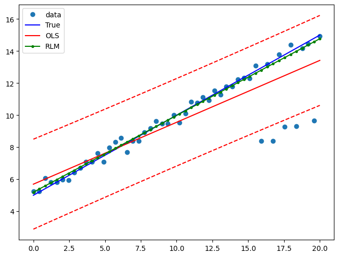
範例 2:具有線性真實值的線性函數
僅使用線性項和常數擬合新的 OLS 模型
[11]:
X2 = X[:, [0, 1]]
res2 = sm.OLS(y2, X2).fit()
print(res2.params)
print(res2.bse)
[5.69278005 0.38633826]
[0.37479982 0.03229427]
估計 RLM
[12]:
resrlm2 = sm.RLM(y2, X2).fit()
print(resrlm2.params)
print(resrlm2.bse)
[5.19360532 0.47898089]
[0.10312091 0.00888531]
繪製圖表以比較 OLS 估計值與穩健估計值
[13]:
pred_ols = res2.get_prediction()
iv_l = pred_ols.summary_frame()["obs_ci_lower"]
iv_u = pred_ols.summary_frame()["obs_ci_upper"]

fig, ax = plt.subplots(figsize=(8, 6))
ax.plot(x1, y2, "o", label="data")
ax.plot(x1, y_true2, "b-", label="True")
ax.plot(x1, res2.fittedvalues, "r-", label="OLS")
ax.plot(x1, iv_u, "r--")
ax.plot(x1, iv_l, "r--")
ax.plot(x1, resrlm2.fittedvalues, "g.-", label="RLM")
legend = ax.legend(loc="best")
上次更新:2024 年 10 月 03 日