Theta 模型
Assimakopoulos & Nikolopoulos (2000) 的 Theta 模型是一種簡單的預測方法,涉及擬合兩條 \(\theta\) 線,使用簡單指數平滑器預測這些線,然後組合兩條線的預測以產生最終預測。該模型按步驟實施:
檢測季節性
若偵測到季節性,則去除季節性
透過將 SES 模型擬合到資料來估計 \(\alpha\),並透過 OLS 估計 \(b_0\)。
預測序列
如果資料已去除季節性,則重新加入季節性。
季節性檢測會檢查季節性延遲 \(m\) 時的 ACF。如果此延遲顯著異於零,則使用 statsmodels.tsa.seasonal_decompose 去除資料的季節性,並使用乘法方法(預設)或加法方法。
模型的參數為 \(b_0\) 和 \(\alpha\),其中 \(b_0\) 是從 OLS 迴歸估計出來的
而 \(\alpha\) 是 SES 中的平滑參數,如下所示:
然後預測為
最終,\(\theta\) 僅在確定趨勢被抑制的程度方面起作用。如果 \(\theta\) 非常大,則模型的預測與帶有漂移的整合移動平均模型的預測相同,
最後,如果需要,將預測重新加入季節性。
此模組基於
Assimakopoulos, V., & Nikolopoulos, K. (2000). The theta model: a decomposition approach to forecasting. International journal of forecasting, 16(4), 521-530.
Hyndman, R. J., & Billah, B. (2003). Unmasking the Theta method. International Journal of Forecasting, 19(2), 287-290.
Fioruci, J. A., Pellegrini, T. R., Louzada, F., & Petropoulos, F. (2015). The optimized theta method. arXiv preprint arXiv:1503.03529.
導入
我們從標準的導入集合和對預設 matplotlib 樣式的一些調整開始。
[1]:
import matplotlib.pyplot as plt
import numpy as np
import pandas as pd
import pandas_datareader as pdr
import seaborn as sns

plt.rc("figure", figsize=(16, 8))
plt.rc("font", size=15)
plt.rc("lines", linewidth=3)
sns.set_style("darkgrid")
載入一些資料
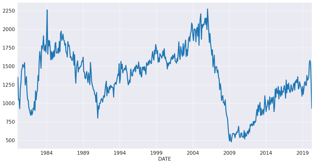
我們將首先使用美國資料查看房屋開工數。這個序列明顯具有季節性,但在相同期間沒有明顯的趨勢。
[2]:
reader = pdr.fred.FredReader(["HOUST"], start="1980-01-01", end="2020-04-01")
data = reader.read()
housing = data.HOUST
housing.index.freq = housing.index.inferred_freq
ax = housing.plot()
我們在沒有任何選項的情況下指定模型並進行擬合。摘要顯示資料已使用乘法方法去除季節性。漂移是適度的且為負值,並且平滑參數相當低。
[3]:
from statsmodels.tsa.forecasting.theta import ThetaModel

tm = ThetaModel(housing)
res = tm.fit()
print(res.summary())
                              ThetaModel Results
==============================================================================
Dep. Variable:                  HOUST   No. Observations:                  484
Method:                       OLS/SES   Deseasonalized:                   True
Date:                Thu, 03 Oct 2024   Deseas. Method:         Multiplicative
Time:                        15:46:28   Period:                             12
Sample:                    01-01-1980
                         - 04-01-2020
   Parameter Estimates
=========================
           Parameters
-------------------------
b0    -0.9194460961668147
alpha   0.616996789006705
-------------------------
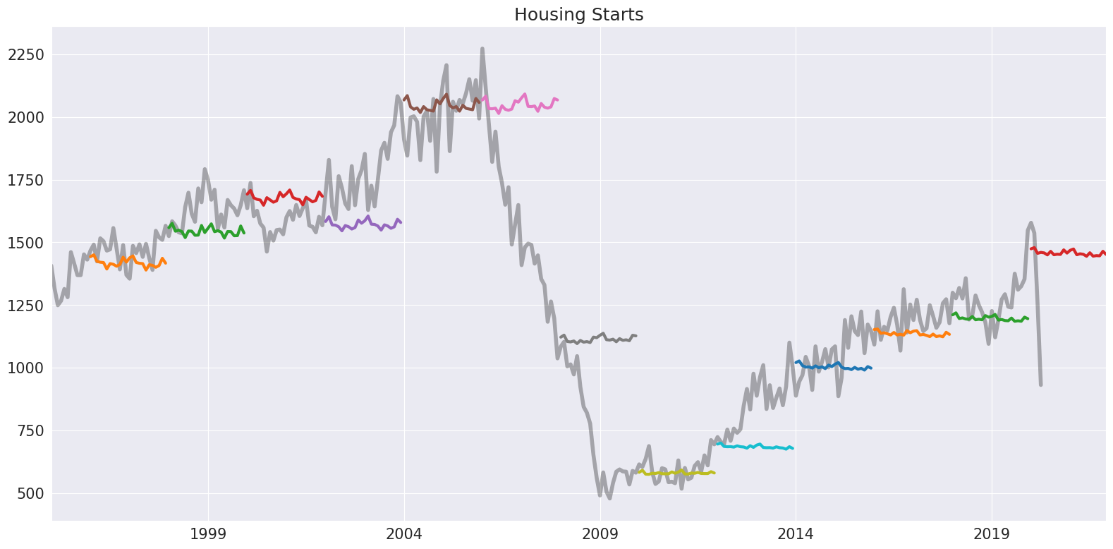
該模型首先是一種預測方法。預測是使用已擬合模型的 forecast 方法產生的。以下我們透過每 2 年預測 2 年來產生一個刺蝟圖。
注意:預設 \(\theta\) 為 2。
[4]:
forecasts = {"housing": housing}
for year in range(1995, 2020, 2):
    sub = housing[: str(year)]
    res = ThetaModel(sub).fit()
    fcast = res.forecast(24)
    forecasts[str(year)] = fcast
forecasts = pd.DataFrame(forecasts)
ax = forecasts["1995":].plot(legend=False)
children = ax.get_children()
children[0].set_linewidth(4)
children[0].set_alpha(0.3)
children[0].set_color("#000000")
ax.set_title("Housing Starts")
plt.tight_layout(pad=1.0)
我們可以選擇擬合資料的對數。在這裡,如果需要,強制去除季節性使用加法方法更有意義。我們還使用 MLE 擬合模型參數。此方法擬合 IMA
其中 \(\hat{\alpha}\) = \(\min(\hat{\gamma}+1, 0.9998)\),使用 statsmodels.tsa.SARIMAX。參數相似,儘管漂移更接近於零。
[5]:
tm = ThetaModel(np.log(housing), method="additive")
res = tm.fit(use_mle=True)
print(res.summary())
                              ThetaModel Results
==============================================================================
Dep. Variable:                  HOUST   No. Observations:                  484
Method:                           MLE   Deseasonalized:                   True
Date:                Thu, 03 Oct 2024   Deseas. Method:               Additive
Time:                        15:46:30   Period:                             12
Sample:                    01-01-1980
                         - 04-01-2020
     Parameter Estimates
=============================
             Parameters
-----------------------------
b0    -0.00044644118691643226
alpha       0.670610385005854
-----------------------------
預測僅取決於預測趨勢分量,
來自 SES 的預測(不隨時間範圍變化)以及季節性。這三個分量可使用 forecast_components 取得。這允許使用上面的權重表達式,以多種 \(\theta\) 選擇來建立預測。
[6]:
res.forecast_components(12)
[6]:
| 趨勢 | ses | 季節性 | |
|---|---|---|---|
| 2020-05-01 | -0.000666 | 6.95726 | -0.001252 |
| 2020-06-01 | -0.001112 | 6.95726 | -0.006891 |
| 2020-07-01 | -0.001559 | 6.95726 | 0.002992 |
| 2020-08-01 | -0.002005 | 6.95726 | -0.003817 |
| 2020-09-01 | -0.002451 | 6.95726 | -0.003902 |
| 2020-10-01 | -0.002898 | 6.95726 | -0.003981 |
| 2020-11-01 | -0.003344 | 6.95726 | 0.008536 |
| 2020-12-01 | -0.003791 | 6.95726 | -0.000714 |
| 2021-01-01 | -0.004237 | 6.95726 | 0.005239 |
| 2021-02-01 | -0.004684 | 6.95726 | 0.009943 |
| 2021-03-01 | -0.005130 | 6.95726 | -0.004535 |
| 2021-04-01 | -0.005577 | 6.95726 | -0.001619 |
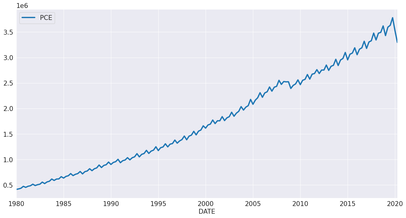
個人消費支出
接下來,我們來看個人消費支出。此序列具有明顯的季節性分量和漂移。
[7]:
reader = pdr.fred.FredReader(["NA000349Q"], start="1980-01-01", end="2020-04-01")
pce = reader.read()
pce.columns = ["PCE"]
pce.index.freq = "QS-OCT"
_ = pce.plot()
由於此序列始終為正值,因此我們對 \(\ln\) 建模。
[8]:
mod = ThetaModel(np.log(pce))
res = mod.fit()
print(res.summary())
                              ThetaModel Results
==============================================================================
Dep. Variable:                    PCE   No. Observations:                  162
Method:                       OLS/SES   Deseasonalized:                   True
Date:                Thu, 03 Oct 2024   Deseas. Method:         Multiplicative
Time:                        15:46:32   Period:                              4
Sample:                    01-01-1980
                         - 04-01-2020
   Parameter Estimates
==========================
           Parameters
--------------------------
b0    0.013035370221488518
alpha   0.9998851279204637
--------------------------
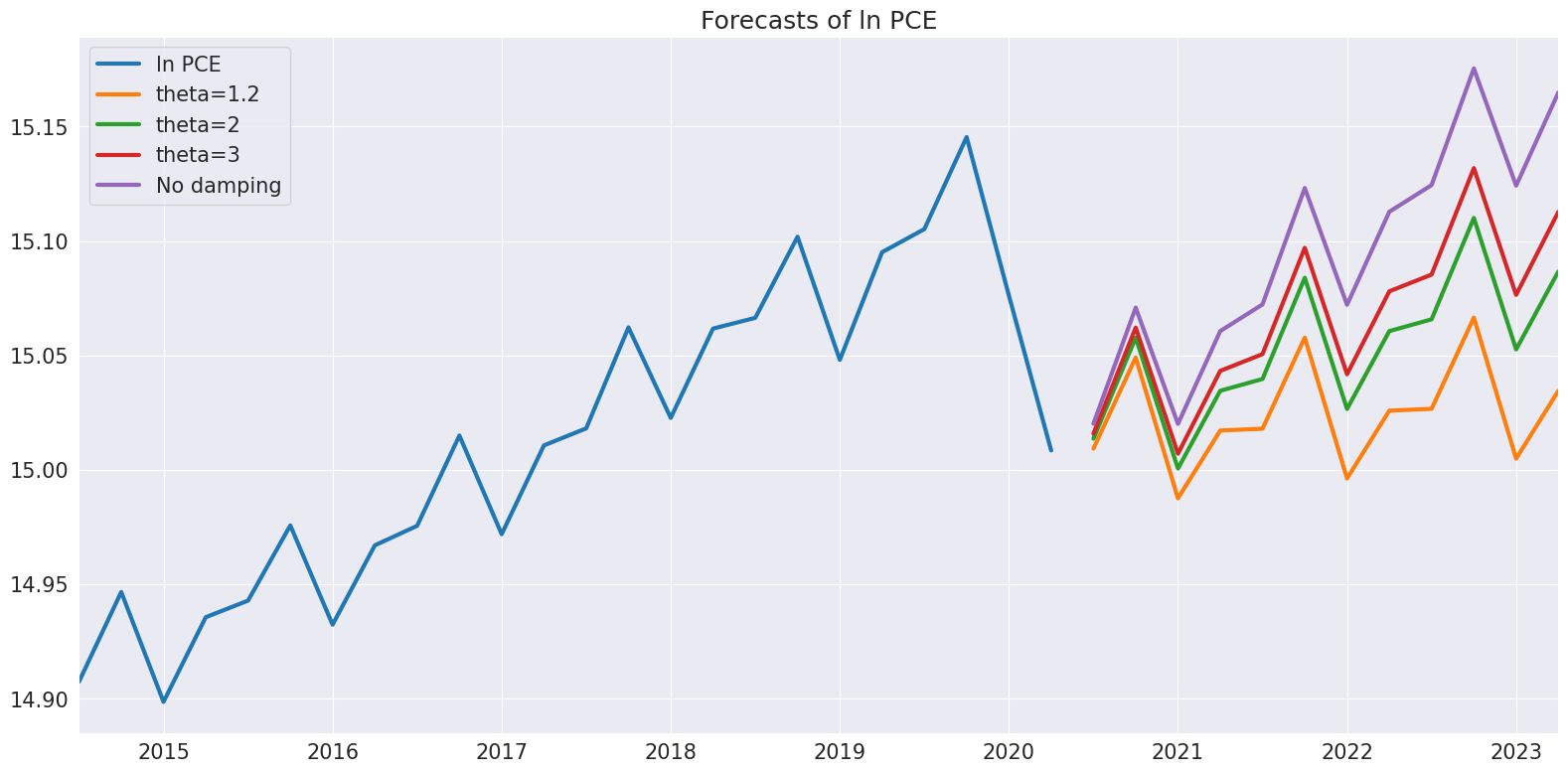
接下來,我們探討預測中的差異,因為 \(\theta\) 會改變。當 \(\theta\) 接近 1 時,漂移幾乎不存在。隨著 \(\theta\) 的增加,漂移變得更加明顯。
[9]:
forecasts = pd.DataFrame(
    {
        "ln PCE": np.log(pce.PCE),
        "theta=1.2": res.forecast(12, theta=1.2),
        "theta=2": res.forecast(12),
        "theta=3": res.forecast(12, theta=3),
        "No damping": res.forecast(12, theta=np.inf),
    }
)
_ = forecasts.tail(36).plot()
plt.title("Forecasts of ln PCE")
plt.tight_layout(pad=1.0)
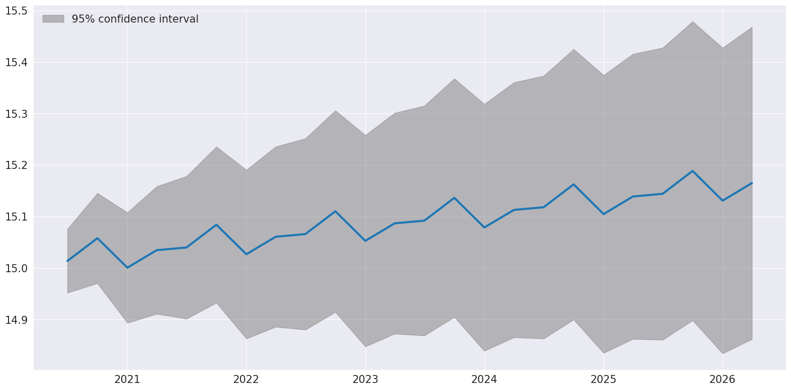
最後,可以使用 plot_predict 來視覺化預測和預測區間,這些預測和預測區間是在假設 IMA 為真的情況下建構的。
[10]:
ax = res.plot_predict(24, theta=2)
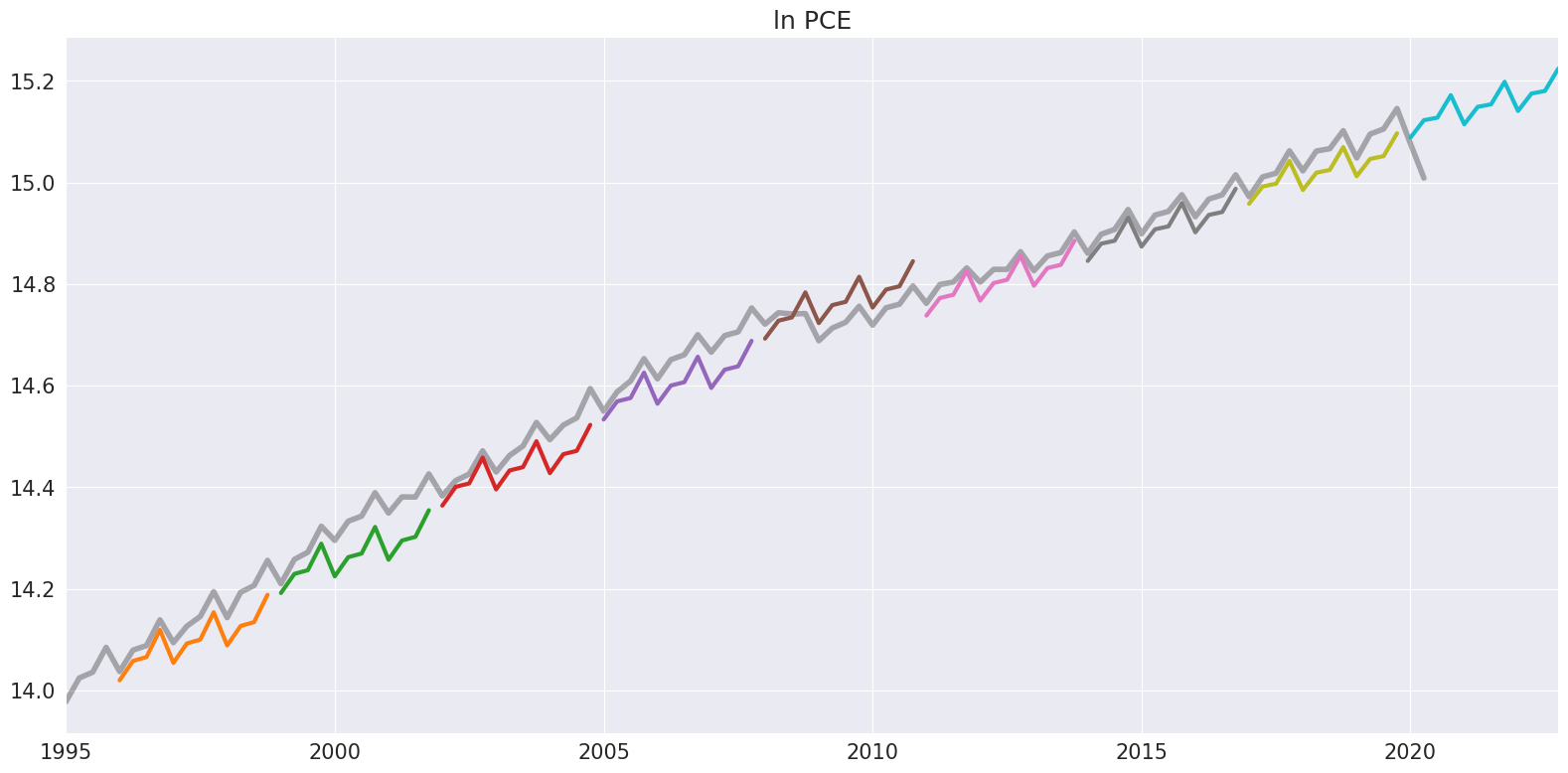
我們最後使用 2 年不重疊的樣本產生一個刺蝟圖。
[11]:
ln_pce = np.log(pce.PCE)
forecasts = {"ln PCE": ln_pce}
for year in range(1995, 2020, 3):
    sub = ln_pce[: str(year)]
    res = ThetaModel(sub).fit()
    fcast = res.forecast(12)
    forecasts[str(year)] = fcast
forecasts = pd.DataFrame(forecasts)
ax = forecasts["1995":].plot(legend=False)
children = ax.get_children()
children[0].set_linewidth(4)
children[0].set_alpha(0.3)
children[0].set_color("#000000")
ax.set_title("ln PCE")
plt.tight_layout(pad=1.0)