迴歸圖
[1]:
%matplotlib inline
[2]:
from statsmodels.compat import lzip
import numpy as np
import matplotlib.pyplot as plt
import statsmodels.api as sm
from statsmodels.formula.api import ols

plt.rc("figure", figsize=(16, 8))
plt.rc("font", size=14)
鄧肯的聲望資料集
載入資料
我們可以使用一個工具函數來載入任何來自優秀的 Rdatasets 套件的 R 資料集。
[3]:
prestige = sm.datasets.get_rdataset("Duncan", "carData", cache=True).data
[4]:
prestige.head()
[4]:
| 類型 | 收入 | 教育程度 | 聲望 | |
|---|---|---|---|---|
| 列名稱 | ||||
| 會計師 | 專業人士 | 62 | 86 | 82 |
| 飛行員 | 專業人士 | 72 | 76 | 83 |
| 建築師 | 專業人士 | 75 | 92 | 90 |
| 作家 | 專業人士 | 55 | 90 | 76 |
| 化學家 | 專業人士 | 64 | 86 | 90 |
[5]:
prestige_model = ols("prestige ~ income + education", data=prestige).fit()
[6]:
print(prestige_model.summary())
                            OLS Regression Results
==============================================================================
Dep. Variable:               prestige   R-squared:                       0.828
Model:                            OLS   Adj. R-squared:                  0.820
Method:                 Least Squares   F-statistic:                     101.2
Date:                Thu, 03 Oct 2024   Prob (F-statistic):           8.65e-17
Time:                        15:58:25   Log-Likelihood:                -178.98
No. Observations:                  45   AIC:                             364.0
Df Residuals:                      42   BIC:                             369.4
Df Model:                           2
Covariance Type:            nonrobust
==============================================================================
                 coef    std err          t      P>|t|      [0.025      0.975]
------------------------------------------------------------------------------
Intercept     -6.0647      4.272     -1.420      0.163     -14.686       2.556
income         0.5987      0.120      5.003      0.000       0.357       0.840
education      0.5458      0.098      5.555      0.000       0.348       0.744
==============================================================================
Omnibus:                        1.279   Durbin-Watson:                   1.458
Prob(Omnibus):                  0.528   Jarque-Bera (JB):                0.520
Skew:                           0.155   Prob(JB):                        0.771
Kurtosis:                       3.426   Cond. No.                         163.
==============================================================================

Notes:
[1] Standard Errors assume that the covariance matrix of the errors is correctly specified.
影響圖
影響圖顯示(外部)學生化殘差與每個觀測值以帽矩陣衡量的槓桿作用之間的關係。
外部學生化殘差是通過其標準差縮放的殘差,其中
其中
\(n\) 是觀測值的數量,而 \(p\) 是迴歸量的數量。\(h_{ii}\) 是帽矩陣的第 \(i\) 個對角元素
每個點的影響可以通過 criterion 關鍵字引數來視覺化。選項包括 Cook 距離和 DFFITS,這是兩種衡量影響的指標。
[7]:
fig = sm.graphics.influence_plot(prestige_model, criterion="cooks")
fig.tight_layout(pad=1.0)
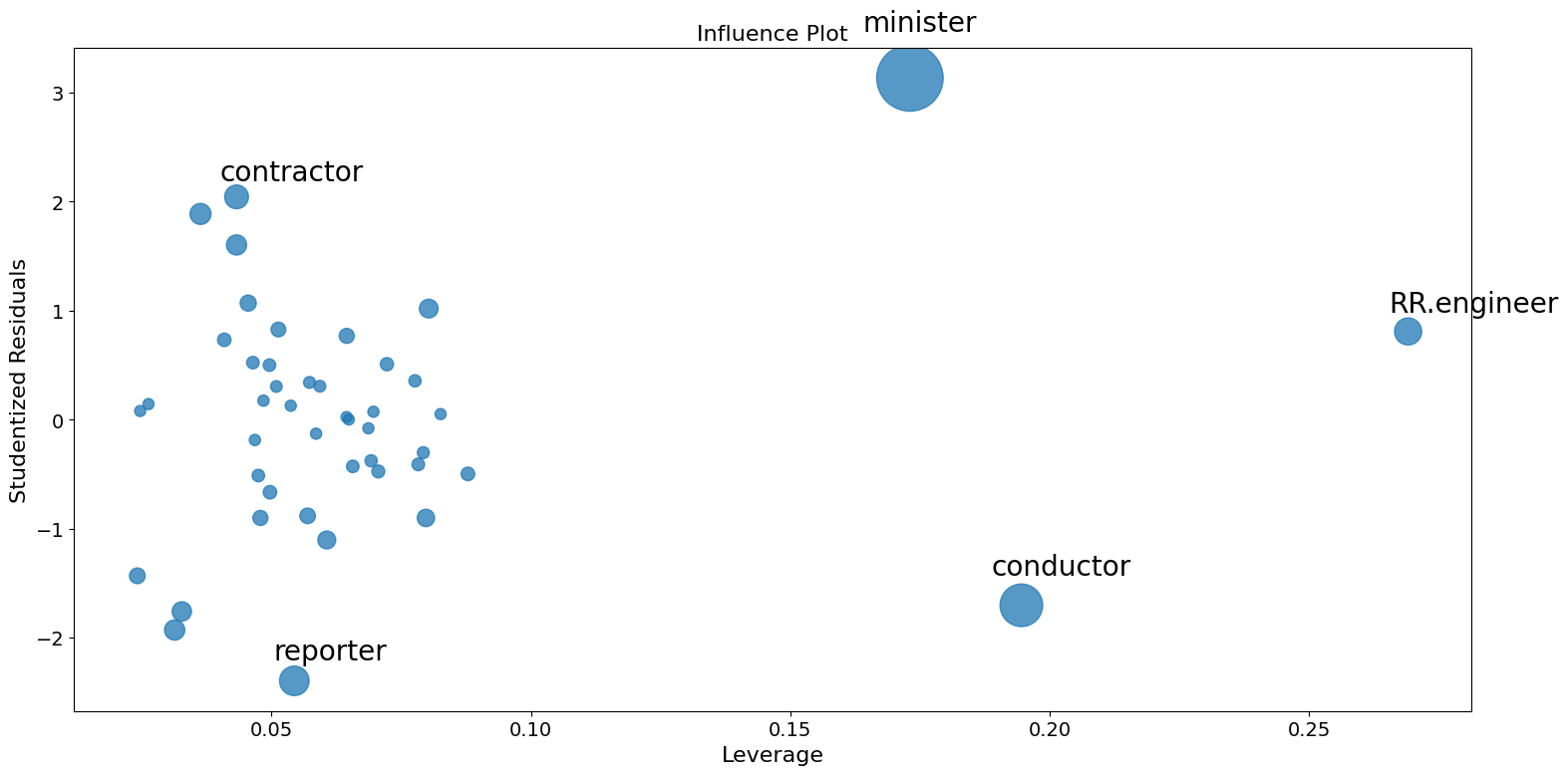
正如你所看到的,有一些令人擔憂的觀察值。承包商和記者都有較低的槓桿作用,但殘差很大。RR.工程師殘差很小,但槓桿作用很大。指揮家和牧師都有很高的槓桿作用和很大的殘差,因此影響很大。
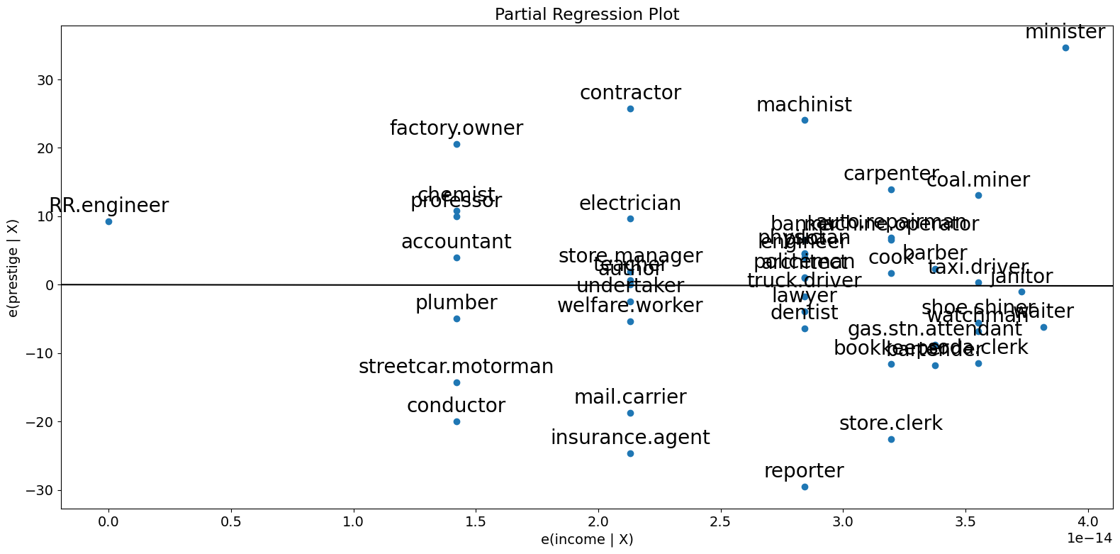
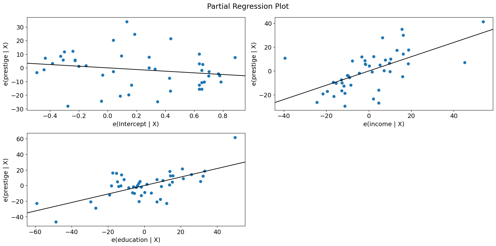
偏迴歸圖 (鄧肯)
由於我們正在進行多變量迴歸,我們不能只看單獨的雙變量圖來辨別關係。相反,我們想要查看在其他自變數條件下,因變數和自變數之間的關係。我們可以通過使用偏迴歸圖來做到這一點,偏迴歸圖也被稱為新增變數圖。
在偏迴歸圖中,為了辨別反應變數和第 \(k\) 個變數之間的關係,我們通過將反應變數對除 \(X_k\) 之外的自變數進行迴歸來計算殘差。我們可以將其表示為 \(X_{\sim k}\)。然後,我們通過將 \(X_k\) 對 \(X_{\sim k}\) 進行迴歸來計算殘差。偏迴歸圖是前者的殘差與後者的殘差的圖。
該圖的顯著點是擬合線的斜率為 \(\beta_k\),截距為零。此圖的殘差與具有完整 \(X\) 的原始模型的最小平方擬合的殘差相同。你可以很容易地辨別出各個資料值對係數估計的影響。如果 obs_labels 為 True,則這些點將使用其觀察標籤進行註釋。你還可以查看違反基本假設的情況,例如同質性和線性。
[8]:
fig = sm.graphics.plot_partregress(
    "prestige", "income", ["income", "education"], data=prestige
)
fig.tight_layout(pad=1.0)
[9]:
fig = sm.graphics.plot_partregress("prestige", "income", ["education"], data=prestige)
fig.tight_layout(pad=1.0)
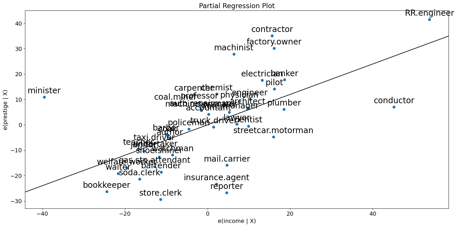
正如你所看到的,偏迴歸圖證實了指揮家、牧師和 RR.工程師對收入和聲望之間偏關係的影響。這些案例大大降低了收入對聲望的影響。刪除這些案例證實了這一點。
[10]:
subset = ~prestige.index.isin(["conductor", "RR.engineer", "minister"])
prestige_model2 = ols(
    "prestige ~ income + education", data=prestige, subset=subset
).fit()
print(prestige_model2.summary())
                            OLS Regression Results
==============================================================================
Dep. Variable:               prestige   R-squared:                       0.876
Model:                            OLS   Adj. R-squared:                  0.870
Method:                 Least Squares   F-statistic:                     138.1
Date:                Thu, 03 Oct 2024   Prob (F-statistic):           2.02e-18
Time:                        15:58:28   Log-Likelihood:                -160.59
No. Observations:                  42   AIC:                             327.2
Df Residuals:                      39   BIC:                             332.4
Df Model:                           2
Covariance Type:            nonrobust
==============================================================================
                 coef    std err          t      P>|t|      [0.025      0.975]
------------------------------------------------------------------------------
Intercept     -6.3174      3.680     -1.717      0.094     -13.760       1.125
income         0.9307      0.154      6.053      0.000       0.620       1.242
education      0.2846      0.121      2.345      0.024       0.039       0.530
==============================================================================
Omnibus:                        3.811   Durbin-Watson:                   1.468
Prob(Omnibus):                  0.149   Jarque-Bera (JB):                2.802
Skew:                          -0.614   Prob(JB):                        0.246
Kurtosis:                       3.303   Cond. No.                         158.
==============================================================================

Notes:
[1] Standard Errors assume that the covariance matrix of the errors is correctly specified.
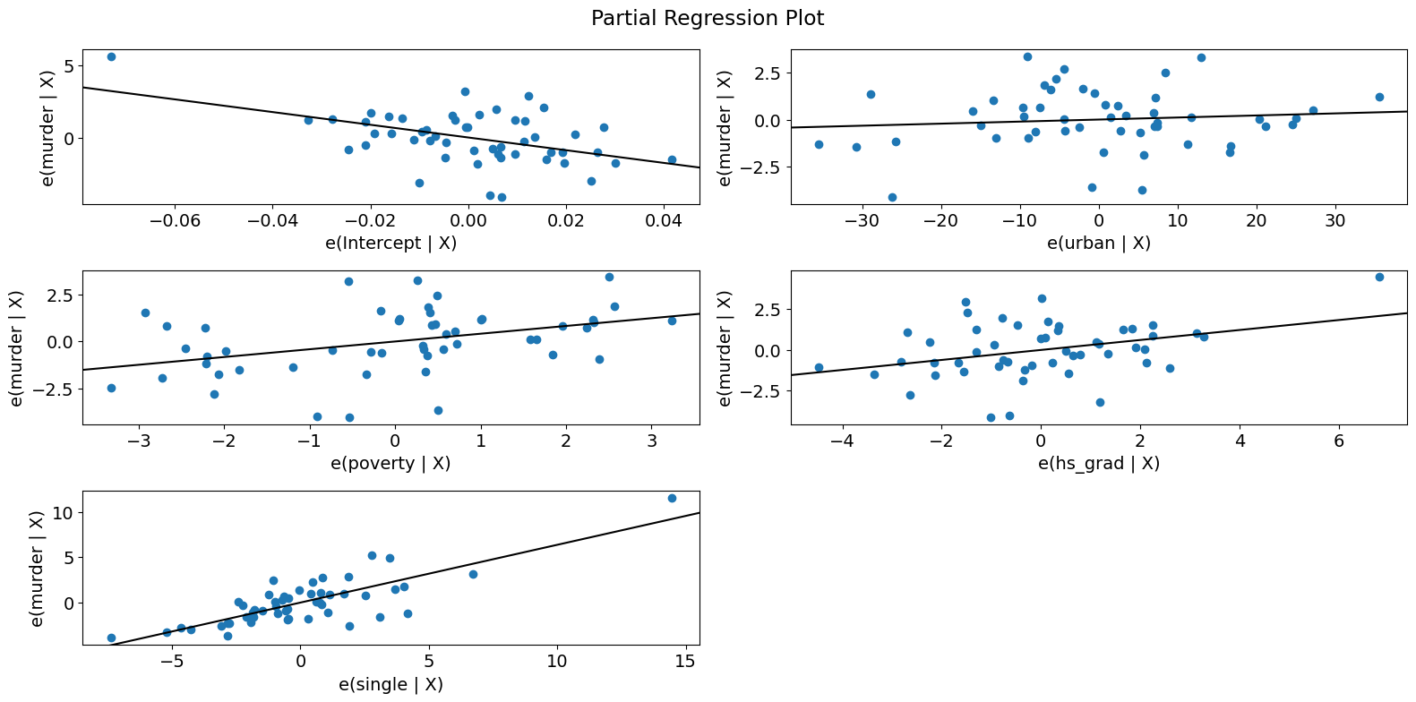
為了快速檢查所有迴歸量,你可以使用 plot_partregress_grid。這些圖不會標記點,但你可以使用它們來識別問題,然後使用 plot_partregress 來獲取更多資訊。
[11]:
fig = sm.graphics.plot_partregress_grid(prestige_model)
fig.tight_layout(pad=1.0)
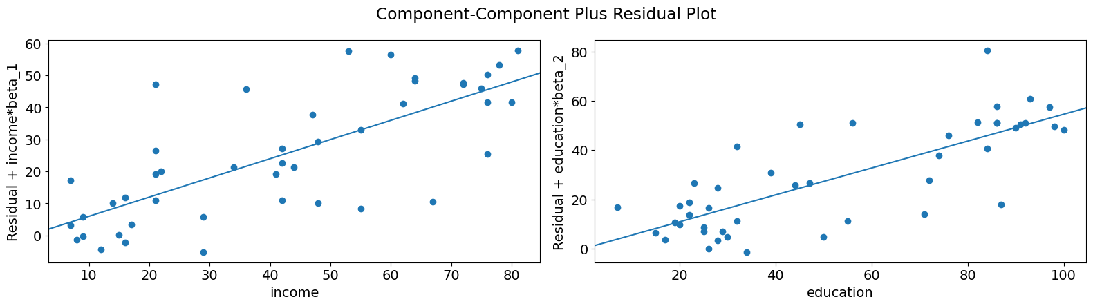
成分-成分加殘差 (CCPR) 圖
CCPR 圖提供了一種方法,通過考慮其他自變數的影響來判斷一個迴歸量對反應變數的影響。偏殘差圖定義為 \(\text{Residuals} + B_iX_i \text{ }\text{ }\) 與 \(X_i\) 的關係。成分將 \(B_iX_i\) 與 \(X_i\) 的關係相加,以顯示擬合線的位置。如果 \(X_i\) 與任何其他自變數高度相關,則應謹慎處理。如果是這種情況,則圖中顯示的變異數將低估真實變異數。
[12]:
fig = sm.graphics.plot_ccpr(prestige_model, "education")
fig.tight_layout(pad=1.0)
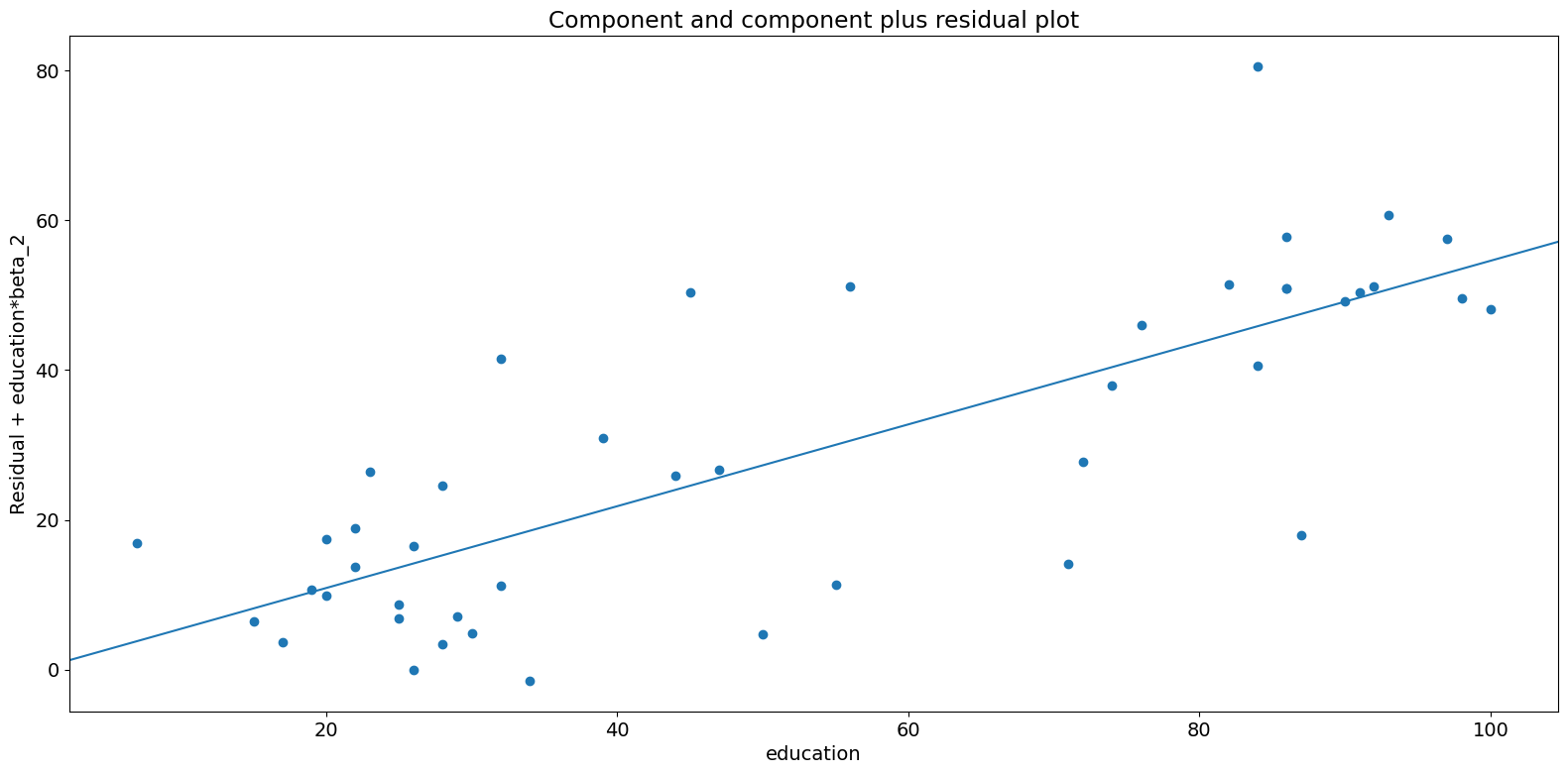
正如你所看到的,在收入的條件下,教育解釋的聲望變異數之間的關係似乎是線性的,儘管你可以看到有一些觀測值對這種關係產生了相當大的影響。我們可以通過使用 plot_ccpr_grid 快速查看多個變數。
[13]:
fig = sm.graphics.plot_ccpr_grid(prestige_model)
fig.tight_layout(pad=1.0)
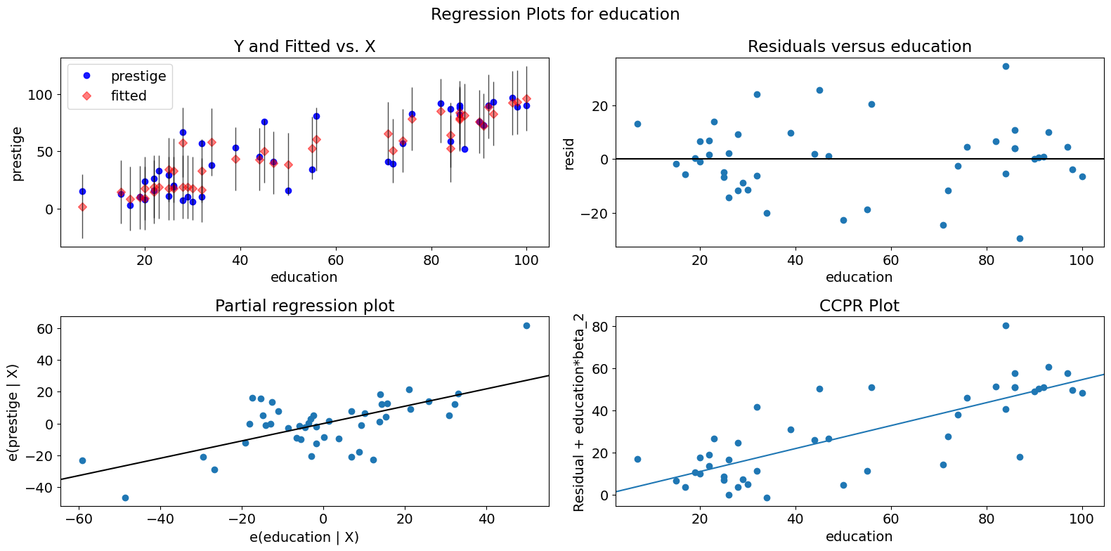
單變數迴歸診斷
plot_regress_exog 函數是一個方便的函數,它提供了一個 2x2 的圖,其中包含因變數和擬合值,以及置信區間與所選的自變數、模型的殘差與所選的自變數、偏迴歸圖和 CCPR 圖。此函數可用於快速檢查與單個迴歸量相關的模型假設。
[14]:
fig = sm.graphics.plot_regress_exog(prestige_model, "education")
fig.tight_layout(pad=1.0)
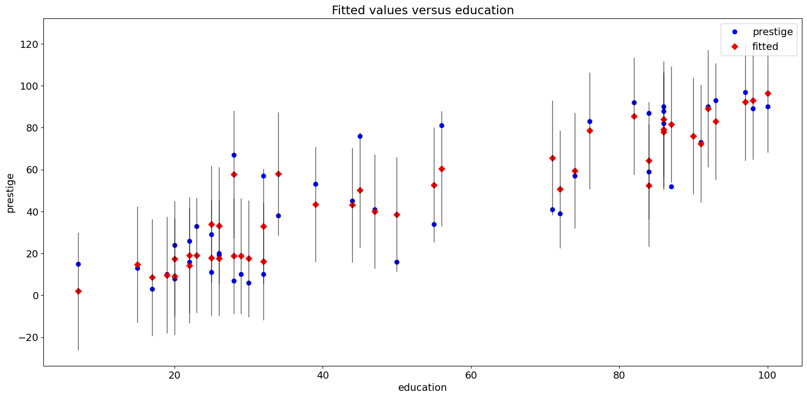
擬合圖
plot_fit 函數繪製擬合值與所選自變數的關係圖。它包括預測置信區間,並且可以選擇繪製真實的因變數。
[15]:
fig = sm.graphics.plot_fit(prestige_model, "education")
fig.tight_layout(pad=1.0)
2009 年全州犯罪資料集
將以下內容與 http://www.ats.ucla.edu/stat/stata/webbooks/reg/chapter4/statareg_self_assessment_answers4.htm 進行比較
儘管此處的資料與該範例中的資料不同。你可以通過取消註釋下面的必要單元來執行該範例。
[16]:
# dta = pd.read_csv("http://www.stat.ufl.edu/~aa/social/csv_files/statewide-crime-2.csv")
# dta = dta.set_index("State", inplace=True).dropna()
# dta.rename(columns={"VR" : "crime",
#                    "MR" : "murder",
#                    "M"  : "pctmetro",
#                    "W"  : "pctwhite",
#                    "H"  : "pcths",
#                    "P"  : "poverty",
#                    "S"  : "single"
#                    }, inplace=True)
#
# crime_model = ols("murder ~ pctmetro + poverty + pcths + single", data=dta).fit()
[17]:
dta = sm.datasets.statecrime.load_pandas().data
[18]:
crime_model = ols("murder ~ urban + poverty + hs_grad + single", data=dta).fit()
print(crime_model.summary())
                            OLS Regression Results
==============================================================================
Dep. Variable:                 murder   R-squared:                       0.813
Model:                            OLS   Adj. R-squared:                  0.797
Method:                 Least Squares   F-statistic:                     50.08
Date:                Thu, 03 Oct 2024   Prob (F-statistic):           3.42e-16
Time:                        15:58:34   Log-Likelihood:                -95.050
No. Observations:                  51   AIC:                             200.1
Df Residuals:                      46   BIC:                             209.8
Df Model:                           4
Covariance Type:            nonrobust
==============================================================================
                 coef    std err          t      P>|t|      [0.025      0.975]
------------------------------------------------------------------------------
Intercept    -44.1024     12.086     -3.649      0.001     -68.430     -19.774
urban          0.0109      0.015      0.707      0.483      -0.020       0.042
poverty        0.4121      0.140      2.939      0.005       0.130       0.694
hs_grad        0.3059      0.117      2.611      0.012       0.070       0.542
single         0.6374      0.070      9.065      0.000       0.496       0.779
==============================================================================
Omnibus:                        1.618   Durbin-Watson:                   2.507
Prob(Omnibus):                  0.445   Jarque-Bera (JB):                0.831
Skew:                          -0.220   Prob(JB):                        0.660
Kurtosis:                       3.445   Cond. No.                     5.80e+03
==============================================================================

Notes:
[1] Standard Errors assume that the covariance matrix of the errors is correctly specified.
[2] The condition number is large, 5.8e+03. This might indicate that there are
strong multicollinearity or other numerical problems.
偏迴歸圖 (犯罪資料)
[19]:
fig = sm.graphics.plot_partregress_grid(crime_model)
fig.tight_layout(pad=1.0)
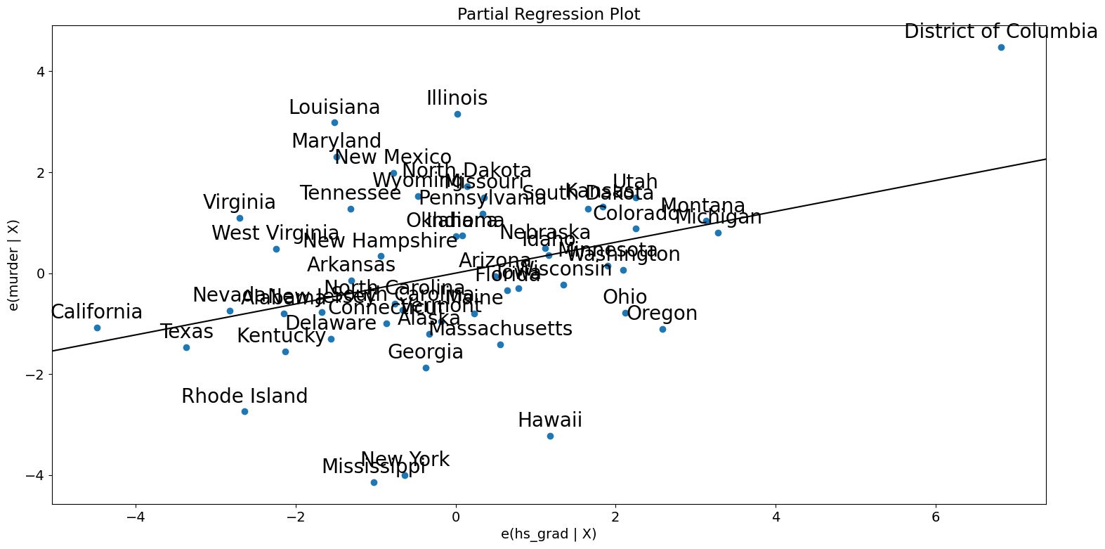
[20]:
fig = sm.graphics.plot_partregress(
    "murder", "hs_grad", ["urban", "poverty", "single"], data=dta
)
fig.tight_layout(pad=1.0)
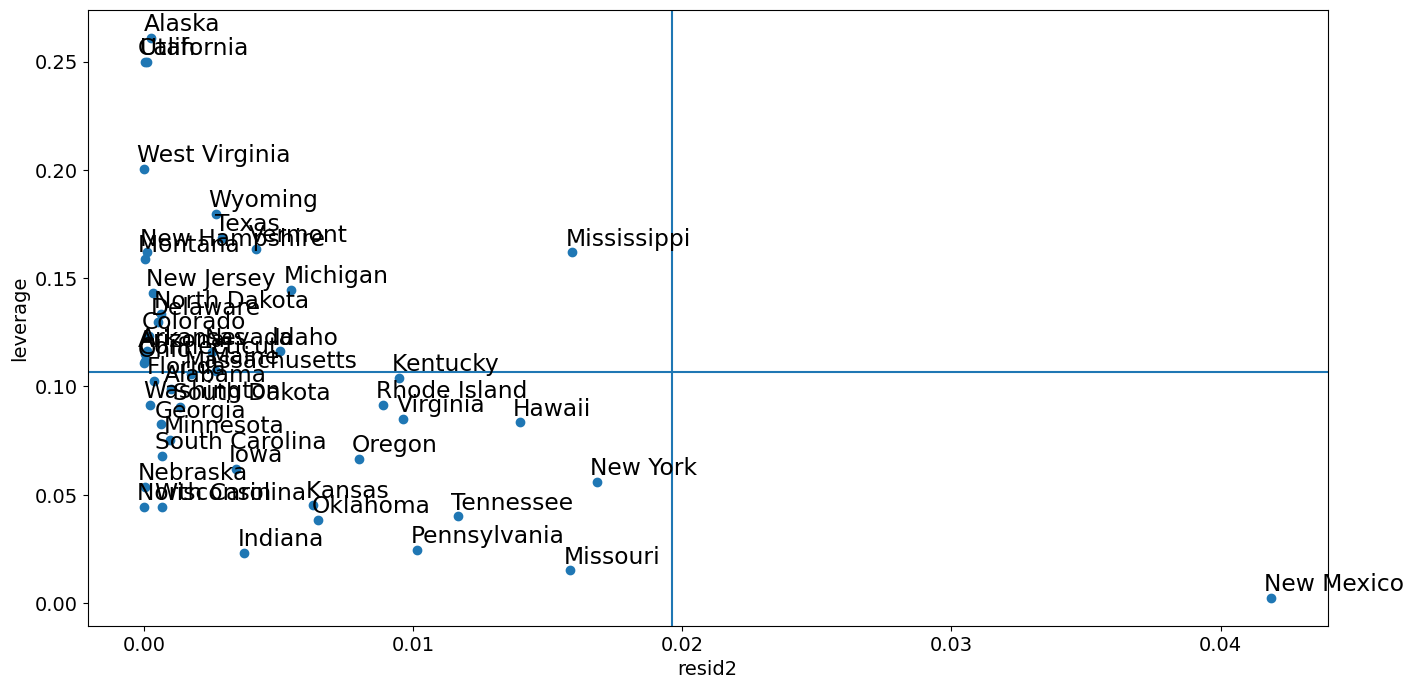
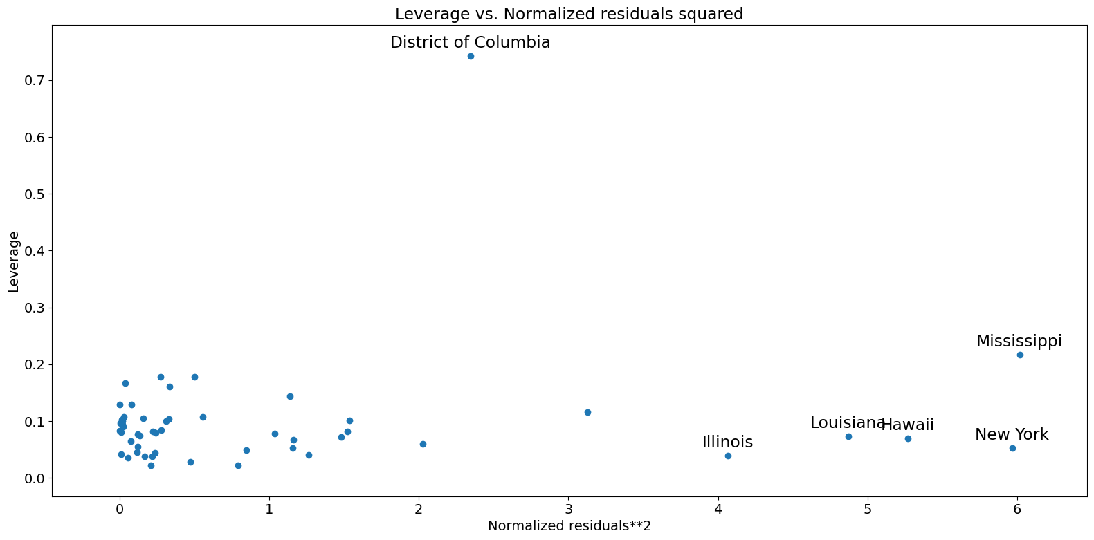
槓桿-殘差平方圖
與 influence_plot 密切相關的是 leverage-resid2 圖。
[21]:
fig = sm.graphics.plot_leverage_resid2(crime_model)
fig.tight_layout(pad=1.0)
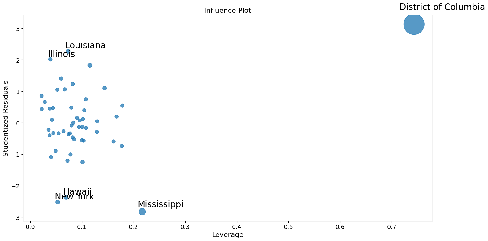
影響圖
[22]:
fig = sm.graphics.influence_plot(crime_model)
fig.tight_layout(pad=1.0)
使用穩健迴歸校正離群值。
這裡重現 Stata 結果的部分問題是,M 估計器對槓桿點不穩健。MM 估計器應該在這個範例中做得更好。
[23]:
from statsmodels.formula.api import rlm
[24]:
rob_crime_model = rlm(
    "murder ~ urban + poverty + hs_grad + single",
    data=dta,
    M=sm.robust.norms.TukeyBiweight(3),
).fit(conv="weights")
print(rob_crime_model.summary())
                    Robust linear Model Regression Results
==============================================================================
Dep. Variable:                 murder   No. Observations:                   51
Model:                            RLM   Df Residuals:                       46
Method:                          IRLS   Df Model:                            4
Norm:                   TukeyBiweight
Scale Est.:                       mad
Cov Type:                          H1
Date:                Thu, 03 Oct 2024
Time:                        15:58:38
No. Iterations:                    50
==============================================================================
                 coef    std err          z      P>|z|      [0.025      0.975]
------------------------------------------------------------------------------
Intercept     -4.2986      9.494     -0.453      0.651     -22.907      14.310
urban          0.0029      0.012      0.241      0.809      -0.021       0.027
poverty        0.2753      0.110      2.499      0.012       0.059       0.491
hs_grad       -0.0302      0.092     -0.328      0.743      -0.211       0.150
single         0.2902      0.055      5.253      0.000       0.182       0.398
==============================================================================

If the model instance has been used for another fit with different fit parameters, then the fit options might not be the correct ones anymore .
[25]:
# rob_crime_model = rlm("murder ~ pctmetro + poverty + pcths + single", data=dta, M=sm.robust.norms.TukeyBiweight()).fit(conv="weights")
# print(rob_crime_model.summary())
RLM 中尚沒有作為影響診斷方法的一部分,但我們可以重新建立它們。(這取決於 issue #888 的狀態)
[26]:
weights = rob_crime_model.weights
idx = weights > 0
X = rob_crime_model.model.exog[idx.values]
ww = weights[idx] / weights[idx].mean()
hat_matrix_diag = ww * (X * np.linalg.pinv(X).T).sum(1)
resid = rob_crime_model.resid
resid2 = resid ** 2
resid2 /= resid2.sum()
nobs = int(idx.sum())
hm = hat_matrix_diag.mean()
rm = resid2.mean()
[27]:
from statsmodels.graphics import utils

fig, ax = plt.subplots(figsize=(16, 8))
ax.plot(resid2[idx], hat_matrix_diag, "o")
ax = utils.annotate_axes(
    range(nobs),
    labels=rob_crime_model.model.data.row_labels[idx],
    points=lzip(resid2[idx], hat_matrix_diag),
    offset_points=[(-5, 5)] * nobs,
    size="large",
    ax=ax,
)
ax.set_xlabel("resid2")
ax.set_ylabel("leverage")
ylim = ax.get_ylim()
ax.vlines(rm, *ylim)
xlim = ax.get_xlim()
ax.hlines(hm, *xlim)
ax.margins(0, 0)