障礙與截斷計數模型¶

作者：Josef Perktold

Statsmodels 現在有了障礙和截斷計數模型，在 0.14 版中新增。

障礙模型由一個針對零的模型和一個針對大於零的計數分佈的模型組成。零模型是一個二元模型，用於區分零計數和大於零的計數。非零計數的計數模型是一個零截斷計數模型。

Statsmodels 目前支援以 Poisson 和負二項式分佈作為零模型和計數模型的障礙模型。二元模型（如 Logit、Probit 或 GLM-二項式）尚不支援作為零模型。Poisson-Poisson 障礙模型的優點是標準 Poisson 模型在兩個模型中具有相同的參數，是一種特殊情況。這為針對 Poisson 模型的障礙模型提供了簡單的 Wald 檢定。

已實作的二元模型是一個設限模型，其中觀測值在 1 處右設限。這表示僅觀察到 0 或 1 個計數。

障礙模型可以透過分別估計零模型和零截斷資料的計數模型來估計，假設觀測值是獨立分佈的（觀測值之間沒有相關性）。參數估計的結果共變異數矩陣是區塊對角矩陣，對角區塊由子模型給定。聯合估計尚未實作。

設限和截斷計數模型的主要開發目的是支援障礙模型。然而，左截斷計數模型除了支援障礙模型外，還有其他應用。右設限模型沒有單獨的意義，因為它們僅支援可以使用 GLM-二項式、Logit 或 Probit 建模的二元觀測值。

對於障礙模型，有一個單一類別 HurdleCountModel，其中包含子模型的分佈作為選項。截斷模型的類別目前為 TruncatedLFPoisson 和 TruncatedLFNegativeBinomialP，其中 “LF” 代表在固定、獨立於觀測值的截斷點處的左截斷。

[ ]:

[1]:

import numpy as np
import pandas as pd

import statsmodels.discrete.truncated_model as smtc

from statsmodels.discrete.discrete_model import (
    Poisson, NegativeBinomial, NegativeBinomialP, GeneralizedPoisson)
from statsmodels.discrete.count_model import (
    ZeroInflatedPoisson,
    ZeroInflatedGeneralizedPoisson,
    ZeroInflatedNegativeBinomialP
    )

from statsmodels.discrete.truncated_model import (
    TruncatedLFPoisson,
    TruncatedLFNegativeBinomialP,
    _RCensoredPoisson,
    HurdleCountModel,
    )

模擬障礙模型¶

我們正在明確模擬 Poisson-Poisson 障礙模型，因為目前沒有任何分佈輔助函式來執行此操作。

[2]:

np.random.seed(987456348)
# large sample to get strong results
nobs = 5000
x = np.column_stack((np.ones(nobs), np.linspace(0, 1, nobs)))

mu0 = np.exp(0.5 *2 * x.sum(1))
y = np.random.poisson(mu0, size=nobs)
print(np.bincount(y))
y_ = y
indices = np.arange(len(y))
mask = mask0 = y > 0
for _ in range(10):

    print( mask.sum())
    indices = mask #indices[mask]
    if not np.any(mask):
        break
    mu_ = np.exp(0.5 * x[indices].sum(1))
    y[indices] = y_ = np.random.poisson(mu_, size=len(mu_))
    np.place(y, mask, y_)
    mask = np.logical_and(mask0, y == 0)

np.bincount(y)

[102 335 590 770 816 739 573 402 265 176 116  59  35   7  11   4]
4898
602
93
11
2
0

[2]:

array([ 102, 1448, 1502, 1049,  542,  234,   81,   31,    6,    5])

估計錯誤指定的 Poisson 模型¶

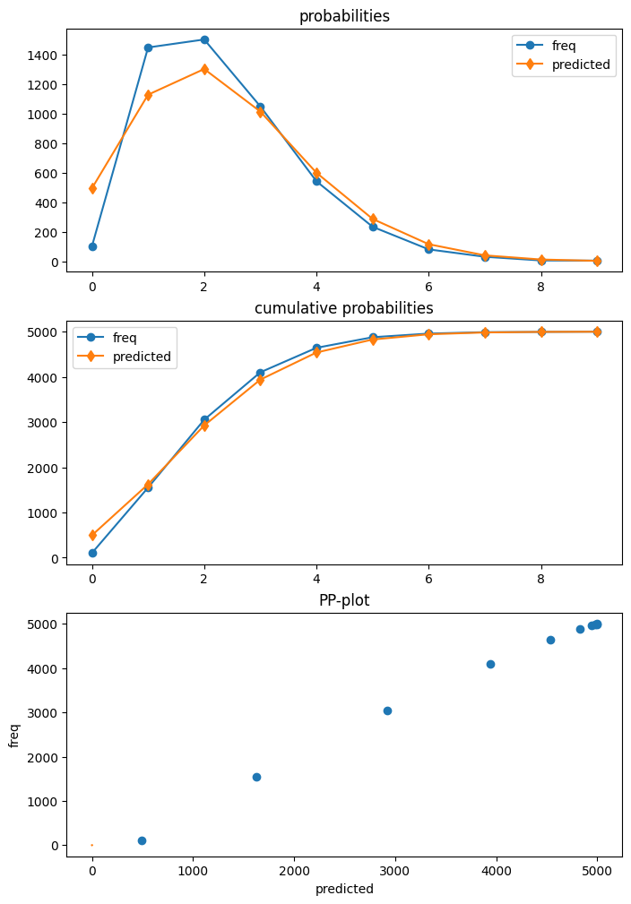
我們產生的資料具有零縮減，也就是說，我們觀察到的零少於我們在 Poisson 模型中預期的零。

在擬合模型之後，我們可以使用 Poisson 診斷類別中的繪圖函式來比較預期的預測分佈和實現的頻率。這顯示 Poisson 模型高估了零的數量，並低估了 1 和 2 的計數。

[3]:

mod_p = Poisson(y, x)
res_p = mod_p.fit()
print(res_p.summary())

Optimization terminated successfully.
         Current function value: 1.668079
         Iterations 4
                          Poisson Regression Results
==============================================================================
Dep. Variable:                      y   No. Observations:                 5000
Model:                        Poisson   Df Residuals:                     4998
Method:                           MLE   Df Model:                            1
Date:                Thu, 03 Oct 2024   Pseudo R-squ.:                0.008678
Time:                        15:44:58   Log-Likelihood:                -8340.4
converged:                       True   LL-Null:                       -8413.4
Covariance Type:            nonrobust   LLR p-value:                 1.279e-33
==============================================================================
                 coef    std err          z      P>|z|      [0.025      0.975]
------------------------------------------------------------------------------
const          0.6532      0.019     33.642      0.000       0.615       0.691
x1             0.3871      0.032     12.062      0.000       0.324       0.450
==============================================================================

[4]:

dia_p = res_p.get_diagnostic()
dia_p.plot_probs();

../../../_images/examples_notebooks_generated_count_hurdle_7_0.png

估計障礙模型¶

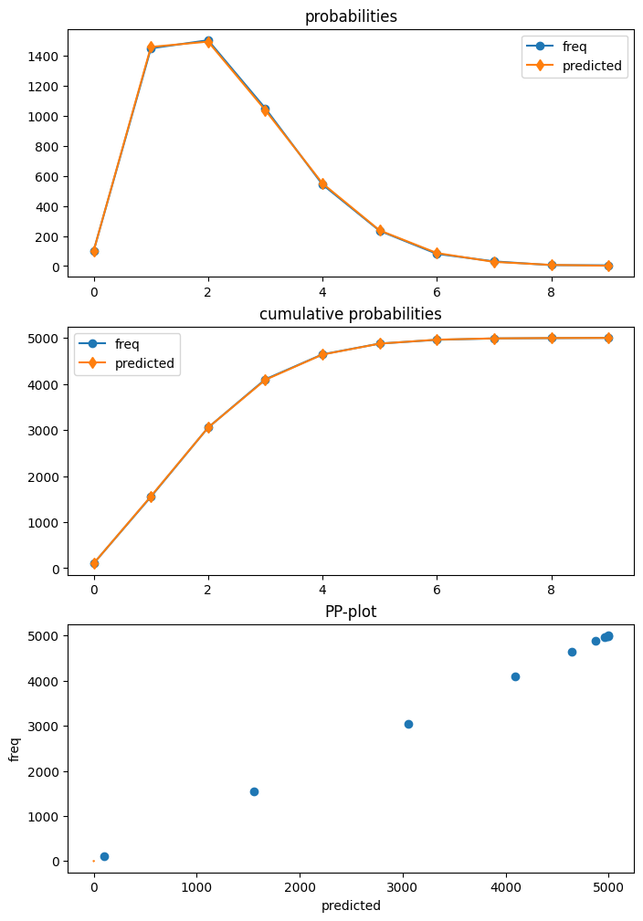
接下來，我們估計正確指定的 Poisson-Poisson 障礙模型。

HurdleCountModel 的簽名和選項顯示 poisson-poisson 是預設值，因此我們在建立此模型時不需要指定任何選項。

HurdleCountModel(endog, exog, offset=None, dist='poisson', zerodist='poisson', p=2, pzero=2, exposure=None, missing='none', **kwargs)

HurdleCountModel 的結果類別有一個 get_diagnostic 方法。但是，目前僅提供部分診斷方法。預測分佈的繪圖顯示與資料非常一致。

[5]:

mod_h = HurdleCountModel(y, x)
res_h = mod_h.fit(disp=False)
print(res_h.summary())

                     HurdleCountModel Regression Results
==============================================================================
Dep. Variable:                      y   No. Observations:                 5000
Model:               HurdleCountModel   Df Residuals:                     4996
Method:                           MLE   Df Model:                            2
Date:                Thu, 03 Oct 2024   Pseudo R-squ.:                 0.01503
Time:                        15:44:59   Log-Likelihood:                -8004.9
converged:               [True, True]   LL-Null:                       -8127.1
Covariance Type:            nonrobust   LLR p-value:                 8.901e-54
==============================================================================
                 coef    std err          z      P>|z|      [0.025      0.975]
------------------------------------------------------------------------------
zm_const       0.9577      0.048     20.063      0.000       0.864       1.051
zm_x1          1.0576      0.121      8.737      0.000       0.820       1.295
const          0.5009      0.024     20.875      0.000       0.454       0.548
x1             0.4577      0.039     11.882      0.000       0.382       0.533
==============================================================================

[6]:

dia_h = res_h.get_diagnostic()
dia_h.plot_probs();

../../../_images/examples_notebooks_generated_count_hurdle_10_0.png

我們可以使用 Wald 檢定來檢定零模型的參數是否與零截斷計數模型的參數相同。p 值非常小，並且正確地拒絕該模型僅為 Poisson 模型。我們正在使用大型樣本大小，因此在這種情況下，檢定的功效將會很大。

[7]:

res_h.wald_test("zm_const = const, zm_x1 = x1", scalar=True)

[7]:

<class 'statsmodels.stats.contrast.ContrastResults'>
<Wald test (chi2): statistic=470.67320754391915, p-value=6.231772522807044e-103, df_denom=2>

預測¶

障礙模型可以用於整體模型和兩個子模型的統計預測。應預測的統計資料是使用 which 關鍵字指定的。

以下摘自 predict 的 docstring，並列出了可用的選項。

which : str (optional)
    Statitistic to predict. Default is 'mean'.

    - 'mean' : the conditional expectation of endog E(y | x)
    - 'mean-main' : mean parameter of truncated count model.
      Note, this is not the mean of the truncated distribution.
    - 'linear' : the linear predictor of the truncated count model.
    - 'var' : returns the estimated variance of endog implied by the
      model.
    - 'prob-main' : probability of selecting the main model which is
      the probability of observing a nonzero count P(y > 0 | x).
    - 'prob-zero' : probability of observing a zero count. P(y=0 | x).
      This is equal to is ``1 - prob-main``
    - 'prob-trunc' : probability of truncation of the truncated count
      model. This is the probability of observing a zero count implied
      by the truncation model.
    - 'mean-nonzero' : expected value conditional on having observation
      larger than zero, E(y | X, y>0)
    - 'prob' : probabilities of each count from 0 to max(endog), or
      for y_values if those are provided. This is a multivariate
      return (2-dim when predicting for several observations).

這些選項在結果類別的 predict 和 get_prediction 方法中可用。

對於以下範例，我們建立一組解釋變數，這些變數取自原始資料，間隔相等。然後，我們可以根據這些解釋變數預測可用的統計資料。

[8]:

which_options = ["mean", "mean-main", "linear", "mean-nonzero", "prob-zero", "prob-main", "prob-trunc", "var", "prob"]
ex = x[slice(None, None, nobs // 5), :]
ex

[8]:

array([[1.        , 0.        ],
       [1.        , 0.20004001],
       [1.        , 0.40008002],
       [1.        , 0.60012002],
       [1.        , 0.80016003]])

[9]:

for w in which_options:
    print(w)
    pred = res_h.predict(ex, which=w)
    print("    ", pred)

mean
     [1.89150663 2.07648059 2.25555158 2.43319456 2.61673457]
mean-main
     [1.65015181 1.8083782  1.98177629 2.17180081 2.38004602]
linear
     [0.50086729 0.59243042 0.68399356 0.77555669 0.86711982]
mean-nonzero
     [2.04231955 2.16292424 2.29857565 2.45116551 2.62277411]
prob-zero
     [0.07384394 0.0399661  0.01871771 0.00733159 0.00230273]
prob-main
     [0.92615606 0.9600339  0.98128229 0.99266841 0.99769727]
prob-trunc
     [0.19202076 0.16391977 0.1378242  0.11397219 0.09254632]
var
     [1.43498239 1.51977118 1.63803729 1.7971727  1.99738345]
prob
     [[7.38439416e-02 3.63208532e-01 2.99674608e-01 1.64836199e-01
  6.80011882e-02 2.24424568e-02 6.17224344e-03 1.45501981e-03
  3.00125448e-04 5.50280612e-05]
 [3.99660987e-02 3.40376213e-01 3.07764462e-01 1.85518182e-01
  8.38717591e-02 3.03343722e-02 9.14266959e-03 2.36191491e-03
  5.33904431e-04 1.07277904e-04]
 [1.87177088e-02 3.10869602e-01 3.08037002e-01 2.03486809e-01
  1.00816333e-01 3.99590837e-02 1.31983274e-02 3.73659033e-03
  9.25635762e-04 2.03822556e-04]
 [7.33159258e-03 2.77316512e-01 3.01138113e-01 2.18003999e-01
  1.18365316e-01 5.14131777e-02 1.86098635e-02 5.77384524e-03
  1.56745522e-03 3.78244503e-04]
 [2.30272798e-03 2.42169151e-01 2.88186862e-01 2.28632665e-01
  1.36039066e-01 6.47558475e-02 2.56869828e-02 8.73374304e-03
  2.59833880e-03 6.87129546e-04]]

[10]:

for w in which_options[:-1]:
    print(w)
    pred = res_h.get_prediction(ex, which=w)
    print("    ", pred.predicted)
    print("  se", pred.se)

mean
     [1.89150663 2.07648059 2.25555158 2.43319456 2.61673457]
  se [0.07877461 0.05693768 0.05866892 0.09551274 0.15359057]
mean-main
     [1.65015181 1.8083782  1.98177629 2.17180081 2.38004602]
  se [0.03959242 0.03164634 0.02471869 0.02415162 0.03453261]
linear
     [0.50086729 0.59243042 0.68399356 0.77555669 0.86711982]
  se [0.04773779 0.03148549 0.02960421 0.04397859 0.06453261]
mean-nonzero
     [2.04231955 2.16292424 2.29857565 2.45116551 2.62277411]
  se [0.02978486 0.02443098 0.01958745 0.0196433  0.02881753]
prob-zero
     [0.07384394 0.0399661  0.01871771 0.00733159 0.00230273]
  se [0.00918583 0.00405155 0.00220446 0.00158494 0.00090255]
prob-main
     [0.92615606 0.9600339  0.98128229 0.99266841 0.99769727]
  se [0.00918583 0.00405155 0.00220446 0.00158494 0.00090255]
prob-trunc
     [0.19202076 0.16391977 0.1378242  0.11397219 0.09254632]
  se [0.00760257 0.00518746 0.00340683 0.00275261 0.00319587]
var
     [1.43498239 1.51977118 1.63803729 1.7971727  1.99738345]
  se [0.04853902 0.03615054 0.02747485 0.02655145 0.03733328]

/opt/hostedtoolcache/Python/3.10.15/x64/lib/python3.10/site-packages/statsmodels/base/_prediction_inference.py:782: UserWarning: using default log-link in get_prediction
  warnings.warn("using default log-link in get_prediction")

選項 which="prob" 會傳回預測機率陣列，用於預測 exog 的每一列。我們通常對所有 exog 的平均機率感興趣。預測方法有一個選項 average=True，用於計算跨觀測值的預測值平均值，以及這些平均預測的對應標準誤差和信賴區間。

[11]:

pred = res_h.get_prediction(ex, which="prob", average=True)
print("    ", pred.predicted)
print("  se", pred.se)

     [2.84324139e-02 3.06788002e-01 3.00960210e-01 2.00095571e-01
 1.01418732e-01 4.17809876e-02 1.45620174e-02 4.41222267e-03
 1.18509193e-03 2.86300514e-04]
  se [2.81472152e-03 5.00830805e-03 1.37524763e-03 1.87343644e-03
 1.99068649e-03 1.23878525e-03 5.78099173e-04 2.21180110e-04
 7.25021189e-05 2.08872558e-05]

我們使用 panda DataFrame 來取得更易於閱讀的顯示。「預測」欄顯示在我們的 5 個 exog 網格點平均的預測回應值分佈的機率質量函式。機率加總不為 1，因為大於觀察到的計數具有正機率，並且在表中遺失，儘管在本範例中該機率很小。

[12]:

dfp_h = pred.summary_frame()
dfp_h

[12]:

	預測	標準誤差	信賴區間下限	信賴區間上限
0	0.028432	0.002815	0.022916	0.033949
1	0.306788	0.005008	0.296972	0.316604
2	0.300960	0.001375	0.298265	0.303656
3	0.200096	0.001873	0.196424	0.203767
4	0.101419	0.001991	0.097517	0.105320
5	0.041781	0.001239	0.039353	0.044209
6	0.014562	0.000578	0.013429	0.015695
7	0.004412	0.000221	0.003979	0.004846
8	0.001185	0.000073	0.001043	0.001327
9	0.000286	0.000021	0.000245	0.000327

[13]:

prob_larger9 = pred.predicted.sum()
prob_larger9, 1 - prob_larger9

[13]:

(np.float64(0.9999215487936677), np.float64(7.84512063323195e-05))

get_prediction 在此情況下會傳回基底 PredictionResultsDelta 類別的實例。

標準誤差、p 值和依賴於數個分佈參數的非線性函式的信賴區間等推論統計資料是使用 delta 方法計算的。預測的推論是基於常態分佈。

[14]:

pred

[14]:

<statsmodels.base._prediction_inference.PredictionResultsDelta at 0x7f68ba217ee0>

[15]:

pred.dist, pred.dist_args

[15]:

(<scipy.stats._continuous_distns.norm_gen at 0x7f68c0dc2a40>, ())

我們可以將障礙模型預測的分佈與我們先前估計的 Poisson 模型預測的分佈進行比較。最後一欄「差異」顯示 Poisson 模型高估了約 8% 觀測值的零數量，並分別在 exog 網格的平均值處低估了 1 和 2 的計數，分別為 7% 和 3.7%。

[16]:

pred_p = res_p.get_prediction(ex, which="prob", average=True)
dfp_p = pred_p.summary_frame()
dfp_h["poisson"] = dfp_p["predicted"]
dfp_h["diff"] = dfp_h["poisson"] - dfp_h["predicted"]
dfp_h

[16]:

	預測	標準誤差	信賴區間下限	信賴區間上限	Poisson	差異
0	0.028432	0.002815	0.022916	0.033949	0.107848	0.079416
1	0.306788	0.005008	0.296972	0.316604	0.237020	-0.069768
2	0.300960	0.001375	0.298265	0.303656	0.263523	-0.037437
3	0.200096	0.001873	0.196424	0.203767	0.197657	-0.002439
4	0.101419	0.001991	0.097517	0.105320	0.112511	0.011093
5	0.041781	0.001239	0.039353	0.044209	0.051833	0.010052
6	0.014562	0.000578	0.013429	0.015695	0.020124	0.005561
7	0.004412	0.000221	0.003979	0.004846	0.006769	0.002356
8	0.001185	0.000073	0.001043	0.001327	0.002012	0.000827
9	0.000286	0.000021	0.000245	0.000327	0.000537	0.000250

其他後估計¶

估計的障礙模型可以用於參數的 Wald 檢定和預測。最大概似統計資料（如對數概似值和資訊準則）也可用。

但是，一些需要輔助函式的後估計方法（對於估計、參數推論和預測而言並非必要）尚未提供。尚未支援的主要方法是 score_test、get_distribution 和 get_influence。get_diagnostics 中的診斷測量僅適用於基於預測的統計資料。

[17]:

res_h.llf, res_h.df_resid, res_h.aic, res_h.bic

[17]:

(np.float64(-8004.904002793644),
 4996,
 np.float64(16017.808005587289),
 np.float64(16043.876778352953))

是否有過度分散？如果模型指定正確，我們可以使用皮爾森殘差來計算應接近 1 的皮爾森 chi2 統計資料。

[18]:

(res_h.resid_pearson**2).sum() / res_h.df_resid

[18]:

np.float64(0.9989670114949286)

診斷類別也具有在診斷圖中使用的預測分佈。目前沒有其他可用的統計資料或檢定。

[19]:

dia_h.probs_predicted.mean(0)

[19]:

array([0.02044612, 0.29147174, 0.29856288, 0.20740118, 0.10990976,
       0.04737579, 0.0172898 , 0.00548983, 0.00154646, 0.00039214])

[20]:

res_h.resid[:10]

[20]:

array([ 1.10849337,  1.10830496, -0.89188344, -0.89207183,  1.10773978,
       -0.8924486 , -0.89263697,  0.10717466,  0.1069863 ,  0.10679794])

[ ]:

上次更新：2024 年 10 月 03 日