後估計概述 - 卜瓦松模型¶

此筆記本提供幾個模型中可用的後估計結果概述，並以卜瓦松模型為例。

另請參閱 https://github.com/statsmodels/statsmodels/issues/7707

傳統上，模型的結果類別提供瓦爾德推論和預測。現在有幾個模型具有用於後估計結果的其他方法，用於推論、預測和規範或診斷檢定。

以下內容基於目前最大概似模型（tsa 之外），主要用於離散模型。其他模型在某種程度上仍然遵循不同的 API 模式。像 OLS 和 WLS 這樣的線性模型有其特殊的實作方式，例如 OLS 影響。GLM 仍然有一些特定於模型的功能。

主要的後估計功能是

推論 - 瓦爾德檢定章節
推論 - 分數檢定章節
get_prediction 包含推論統計的預測章節
get_distribution 基於估計參數的分佈類別章節
get_diagnostic 診斷和規範檢定、度量和繪圖章節
get_influence 離群值和影響診斷章節

警告最近新增的功能不穩定。

主要功能已通過單元測試並與其他統計套件進行驗證。但是，並非每個選項都經過完整測試。隨著新增更多功能，API、選項、預設值和回傳型別仍可能變更。（目前重點是新增功能，而不是尋找方便且面向未來的介面。）

一個模擬範例¶

為了說明，我們模擬卜瓦松迴歸的資料，該迴歸經過正確的設定並具有相對較大的樣本。一個迴歸變數是具有兩個層級的類別變數，第二個迴歸變數在單位區間上均勻分佈。

[1]:

import numpy as np
import pandas as pd
from scipy import stats
import matplotlib.pyplot as plt

from statsmodels.discrete.discrete_model import Poisson
from statsmodels.discrete.diagnostic import PoissonDiagnostic

[2]:

np.random.seed(983154356)

nr = 10
n_groups = 2
labels = np.arange(n_groups)
x = np.repeat(labels, np.array([40, 60]) * nr)
nobs = x.shape[0]
exog = (x[:, None] == labels).astype(np.float64)
xc = np.random.rand(len(x))
exog = np.column_stack((exog, xc))
# reparameterize to explicit constant
# exog[:, 1] = 1
beta = np.array([0.2, 0.3, 0.5], np.float64)

linpred = exog @ beta
mean = np.exp(linpred)
y = np.random.poisson(mean)
len(y), y.mean(), (y == 0).mean()

res = Poisson(y, exog).fit(disp=0)
print(res.summary())

                          Poisson Regression Results
==============================================================================
Dep. Variable:                      y   No. Observations:                 1000
Model:                        Poisson   Df Residuals:                      997
Method:                           MLE   Df Model:                            2
Date:                Thu, 03 Oct 2024   Pseudo R-squ.:                 0.01258
Time:                        15:46:52   Log-Likelihood:                -1618.3
converged:                       True   LL-Null:                       -1638.9
Covariance Type:            nonrobust   LLR p-value:                 1.120e-09
==============================================================================
                 coef    std err          z      P>|z|      [0.025      0.975]
------------------------------------------------------------------------------
x1             0.2386      0.061      3.926      0.000       0.120       0.358
x2             0.3229      0.055      5.873      0.000       0.215       0.431
x3             0.5109      0.083      6.186      0.000       0.349       0.673
==============================================================================

[ ]:

推論 - 瓦爾德檢定¶

瓦爾德檢定和其他推論統計量（例如基於瓦爾德檢定的信賴區間）從一開始就是模型的一個功能。瓦爾德推論基於在估計參數下評估的黑塞矩陣或預期訊息矩陣。

參數的共變異數矩陣可以選擇性地採用三明治形式，該形式對於未指定的異方差或序列或集群相關性具有穩健性（fit 的 cov_type 選項）。

目前可用的方法（除了參數表中的統計量之外）是

t_test
wald_test
t_test_pairwise
wald_test_terms

f_test 可作為傳統方法使用。它與帶有關鍵字選項 use_f=True 的 wald_test 相同。

[3]:

res.t_test("x1=x2")

[3]:

<class 'statsmodels.stats.contrast.ContrastResults'>
                             Test for Constraints
==============================================================================
                 coef    std err          z      P>|z|      [0.025      0.975]
------------------------------------------------------------------------------
c0            -0.0843      0.049     -1.717      0.086      -0.181       0.012
==============================================================================

[4]:

res.wald_test("x1=x2, x3", scalar=True)

[4]:

<class 'statsmodels.stats.contrast.ContrastResults'>
<Wald test (chi2): statistic=40.772322944293464, p-value=1.4008852592190214e-09, df_denom=2>

推論 - score_test¶

statsmodels 0.14 中針對大多數離散模型和 GLM 新增的功能。

分數或拉格朗日乘數 (LM) 檢定基於在虛無假設下估計的模型。一個常見的範例是變數添加檢定，我們在虛無限制下估計模型參數，但針對完整模型評估分數和黑塞矩陣，以檢定額外變數是否具有統計顯著性。

注意： 與瓦爾德檢定類似，離散模型和 GLM 中實作的分數檢定也具有使用異方差或相關性穩健共變異數類型的選項。
它目前使用與瓦爾德檢定相同的實作和預設值來處理穩健共變異數矩陣。在某些情況下，瓦爾德檢定的 cov_type 中包含的小樣本校正不適用於分數檢定。在許多情況下，瓦爾德檢定會過度拒絕，但分數檢定可能會拒絕不足。將瓦爾德小樣本校正用於分數檢定可能會導致更保守的 p 值。
（小樣本校正的預設值未來可能會變更。目前關於異方差和相關性穩健分數檢定的小樣本校正的一般資訊很少。其他統計套件僅針對少數特殊情況實作。）

我們可以使用變數添加分數檢定進行規範檢定。在以下範例中，我們透過添加二次或多項式項來檢定模型中是否存在一些錯誤指定的非線性。

在我們的範例中，我們可以預期這些規範檢定不會拒絕虛無假設，因為模型已正確指定且樣本大小很大。

[5]:

res.score_test(exog_extra=xc**2)

[5]:

(array([0.05300569]), array([0.81791332]), 1)

重設檢定是對連結函數的正確規範的檢定。檢定的標準形式將線性預測器的多項式項作為額外的迴歸變數加入，並檢定它們的顯著性。在這裡，我們使用變數添加分數檢定進行重設檢定，冪次為 2 和 3。

[6]:

linpred = res.predict(which="linear")
res.score_test(exog_extra=linpred[:,None]**[2, 3])

[6]:

(array([1.3867703]), array([0.49988103]), 2)

預測¶

模型和結果類別具有 predict 方法，該方法僅回傳預測值。get_prediction 方法會新增預測的推論統計量、標準誤、p 值和信賴區間。

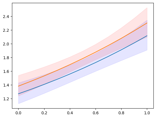
在以下範例中，我們建立新的解釋變數集，這些變數集按類別層級分割並在連續變數的均勻網格上分割。

[7]:

n = 11
exc = np.linspace(0, 1, n)
ex1 = np.column_stack((np.ones(n), np.zeros(n), exc))
ex2 = np.column_stack((np.zeros(n), np.ones(n), exc))

m1 = res.get_prediction(ex1)
m2 = res.get_prediction(ex2)

預測結果類別的可用方法和屬性為

[8]:

[i for i in dir(m1) if not i.startswith("_")]

[8]:

['conf_int',
 'deriv',
 'df',
 'dist',
 'dist_args',
 'func',
 'linpred',
 'linpred_se',
 'predicted',
 'row_labels',
 'se',
 'summary_frame',
 't_test',
 'tvalues',
 'var_pred']

[9]:

plt.plot(exc, np.column_stack([m1.predicted, m2.predicted]))
ci = m1.conf_int()
plt.fill_between(exc, ci[:, 0], ci[:, 1], color='b', alpha=.1)
ci = m2.conf_int()
plt.fill_between(exc, ci[:, 0], ci[:, 1], color='r', alpha=.1)
# to add observed points:
# y1 = y[x == 0]
# plt.plot(xc[x == 0], y1, ".", color="b", alpha=.3)
# y2 = y[x == 1]
# plt.plot(xc[x == 1], y2, ".", color="r", alpha=.3)

[9]:

<matplotlib.collections.PolyCollection at 0x7f852a5340a0>

../../../_images/examples_notebooks_generated_postestimation_poisson_16_1.png

[10]:

y.max()

[10]:

np.int64(7)

我們可以預測的可用統計量之一（由「which」關鍵字指定）是預測分佈的預期頻率或機率。這顯示我們在給定的一組解釋變數下，觀察到計數 = 1、2、3、... 的預測機率是多少。

[11]:

y_max = 5
f1 = res.get_prediction(ex1, which="prob", y_values=np.arange(y_max + 1))
f2 = res.get_prediction(ex2, which="prob", y_values=np.arange(y_max + 1))
f1.predicted.mean(0), f2.predicted.mean(0)

[11]:

(array([0.19681697, 0.31325239, 0.25570764, 0.14275759, 0.06128168,
        0.02154715]),
 array([0.17115113, 0.29529781, 0.26128059, 0.15810937, 0.07357482,
        0.02804883]))

我們也可以取得預測機率的信賴區間。但是，如果我們想要平均預測機率的信賴區間，那麼我們需要在預測函數中彙總。相關關鍵字是「average」，它計算 exog 陣列給定的觀察值上的預測平均值。

[12]:

f1 = res.get_prediction(ex1, which="prob", y_values=np.arange(y_max + 1), average=True)
f2 = res.get_prediction(ex2, which="prob", y_values=np.arange(y_max + 1), average=True)
f1.predicted, f2.predicted

[12]:

(array([0.19681697, 0.31325239, 0.25570764, 0.14275759, 0.06128168,
        0.02154715]),
 array([0.17115113, 0.29529781, 0.26128059, 0.15810937, 0.07357482,
        0.02804883]))

[13]:

f1.conf_int()

[13]:

array([[0.17256941, 0.22106453],
       [0.2982307 , 0.32827408],
       [0.24818616, 0.26322912],
       [0.12876732, 0.15674787],
       [0.05088296, 0.07168041],
       [0.01626921, 0.0268251 ]])

[14]:

f2.conf_int()

[14]:

array([[0.15303084, 0.18927142],
       [0.28178041, 0.30881522],
       [0.25622062, 0.26634055],
       [0.14720224, 0.1690165 ],
       [0.06442055, 0.0827291 ],
       [0.02287077, 0.03322688]])

若要取得關於預測方法和可用選項的更多資訊，請參閱
help(res.get_prediction)
help(res.model.predict)

分佈¶

對於給定的參數，我們可以建立 scipy 或相容於 scipy 的分佈類別的實例。這使我們可以存取分佈中的任何方法，pmf/pdf、cdf、統計量。

結果類別的 get_distribution 方法使用提供的解釋變數陣列和估計參數來指定向量化的分佈。模型的 get_prediction 方法可以用於使用者指定的參數 params。

[15]:

distr = res.get_distribution()
distr

[15]:

<scipy.stats._distn_infrastructure.rv_discrete_frozen at 0x7f852a592e30>

[16]:

distr.pmf(0)[:10]

[16]:

array([0.15420516, 0.13109359, 0.17645042, 0.16735421, 0.13445031,
       0.14851843, 0.22287053, 0.14979318, 0.25252986, 0.25013583])

條件分佈的平均值與模型預測的平均值相同。

[17]:

distr.mean()[:10]

[17]:

array([1.86947133, 2.03184379, 1.73471534, 1.78764267, 2.00656061,
       1.90704623, 1.50116427, 1.89849971, 1.37622577, 1.3857512 ])

[18]:

res.predict()[:10]

[18]:

array([1.86947133, 2.03184379, 1.73471534, 1.78764267, 2.00656061,
       1.90704623, 1.50116427, 1.89849971, 1.37622577, 1.3857512 ])

我們也可以取得一組新的解釋變數的分佈。解釋變數的提供方式與預測方法相同。

我們再次使用預測章節中的解釋變數網格。作為其用法的範例，我們可以計算在解釋變數的值條件下，觀察到（嚴格）大於 5 的計數的機率。

[19]:

distr1 = res.get_distribution(ex1)
distr2 = res.get_distribution(ex2)

[20]:

distr1.sf(5), distr2.sf(5)

[20]:

(array([0.00198421, 0.00255027, 0.00326858, 0.00417683, 0.00532093,
        0.00675641, 0.00854998, 0.01078116, 0.0135439 , 0.01694825,
        0.02112179]),
 array([0.00299758, 0.00383456, 0.00489029, 0.00621677, 0.00787663,
        0.00994468, 0.01250966, 0.01567579, 0.01956437, 0.02431503,
        0.03008666]))

[21]:

plt.plot(exc, np.column_stack([distr1.sf(5), distr2.sf(5)]))

[21]:

[<matplotlib.lines.Line2D at 0x7f852a42cb50>,
 <matplotlib.lines.Line2D at 0x7f852a42cc40>]

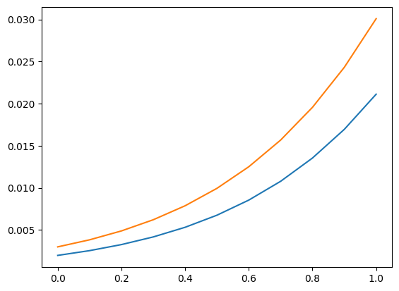
../../../_images/examples_notebooks_generated_postestimation_poisson_34_1.png

我們也可以使用分佈來尋找新的觀察值的上限信賴限值。以下繪圖和表格顯示給定解釋變數的上限計數。觀察到此計數或更少的機率至少為 0.99。

請注意，這將參數視為固定，並且不考慮參數不確定性。

[22]:

plt.plot(exc, np.column_stack([distr1.ppf(0.99), distr2.ppf(0.99)]))

[22]:

[<matplotlib.lines.Line2D at 0x7f852a536140>,
 <matplotlib.lines.Line2D at 0x7f852a5358a0>]

../../../_images/examples_notebooks_generated_postestimation_poisson_36_1.png

[23]:

[distr1.ppf(0.99), distr2.ppf(0.99)]

[23]:

[array([4., 5., 5., 5., 5., 5., 5., 6., 6., 6., 6.]),
 array([5., 5., 5., 5., 5., 5., 6., 6., 6., 6., 6.])]

診斷¶

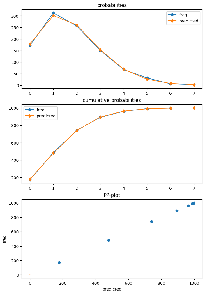
卜瓦松模型是第一個具有診斷類別的模型，可以使用 get_diagnostic 從結果中取得。其他計數模型有一個通用的計數診斷類別，目前只有有限的方法。

在我們的範例中，卜瓦松模型已正確指定。此外，我們有大量的樣本數。因此，在這種情況下，沒有任何診斷檢定會拒絕正確規格的虛無假設。

[24]:

dia = res.get_diagnostic()
[i for i in dir(dia) if not i.startswith("_")]

[24]:

['plot_probs',
 'probs_predicted',
 'results',
 'test_chisquare_prob',
 'test_dispersion',
 'test_poisson_zeroinflation',
 'y_max']

[25]:

dia.plot_probs();

../../../_images/examples_notebooks_generated_postestimation_poisson_40_0.png

檢定過度分散

卜瓦松模型有幾個可用的分散檢定。目前，所有檢定都會回傳結果。 DispersionResults 類別有一個 summary_frame 方法。回傳的資料框架提供了一個更容易閱讀的結果概觀。

[26]:

td = dia.test_dispersion()
td

[26]:

<class 'statsmodels.discrete._diagnostics_count.DispersionResults'>
statistic = array([-0.42597379, -0.42597379, -0.39884024, -0.48327447, -0.48327447,
           -0.47790855, -0.45225818])
pvalue = array([0.67012695, 0.67012695, 0.69001092, 0.62890087, 0.62890087,
           0.6327153 , 0.651083  ])
method = ['Dean A', 'Dean B', 'Dean C', 'CT nb2', 'CT nb1', 'CT nb2 HC3', 'CT nb1 HC3']
alternative = ['mu (1 + a mu)', 'mu (1 + a mu)', 'mu (1 + a)', 'mu (1 + a mu)', 'mu (1 + a)', 'mu (1 + a mu)', 'mu (1 + a)']
name = 'Poisson Dispersion Test'
tuple = (array([-0.42597379, -0.42597379, -0.39884024, -0.48327447, -0.48327447,
           -0.47790855, -0.45225818]), array([0.67012695, 0.67012695, 0.69001092, 0.62890087, 0.62890087,
           0.6327153 , 0.651083  ]))

[27]:

df = td.summary_frame()
df

[27]:

	統計量	p值	方法	對立假設
0	-0.425974	0.670127	Dean A	mu (1 + a mu)
1	-0.425974	0.670127	Dean B	mu (1 + a mu)
2	-0.398840	0.690011	Dean C	mu (1 + a)
3	-0.483274	0.628901	CT nb2	mu (1 + a mu)
4	-0.483274	0.628901	CT nb1	mu (1 + a)
5	-0.477909	0.632715	CT nb2 HC3	mu (1 + a mu)
6	-0.452258	0.651083	CT nb1 HC3	mu (1 + a)

檢定零膨脹

[28]:

dia.test_poisson_zeroinflation()

[28]:

<class 'statsmodels.stats.base.HolderTuple'>
statistic = np.float64(-0.6657556201098714)
pvalue = np.float64(0.5055673158225651)
pvalue_smaller = np.float64(0.7472163420887175)
pvalue_larger = np.float64(0.25278365791128254)
chi2 = np.float64(0.44323054570787945)
pvalue_chi2 = np.float64(0.505567315822565)
df_chi2 = 1
distribution = 'normal'
tuple = (np.float64(-0.6657556201098714), np.float64(0.5055673158225651))

零膨脹的卡方檢定

[29]:

dia.test_chisquare_prob(bin_edges=np.arange(3))

[29]:

<class 'statsmodels.stats.base.HolderTuple'>
statistic = np.float64(0.456170941873113)
pvalue = np.float64(0.4994189468121014)
df = np.int64(1)
diff1 = array([[-0.15420516,  0.71171787],
           [-0.13109359, -0.26636169],
           [-0.17645042, -0.30609125],
           ...,
           [-0.10477112, -0.23636125],
           [-0.10675436, -0.2388335 ],
           [-0.21168332, -0.32867305]])
res_aux = <statsmodels.regression.linear_model.RegressionResultsWrapper object at 0x7f852a290eb0>
distribution = 'chi2'
tuple = (np.float64(0.456170941873113), np.float64(0.4994189468121014))

預測頻率的適合度檢定

這是一個卡方檢定，其中考慮了參數是估計的。大於最大組距邊界的計數將被加到最後一個組距，以便組距的總和為一。

例如，使用 5 個組距

[30]:

dt = dia.test_chisquare_prob(bin_edges=np.arange(6))
dt

[30]:

<class 'statsmodels.stats.base.HolderTuple'>
statistic = np.float64(0.9414641297779136)
pvalue = np.float64(0.9185382008345917)
df = np.int64(4)
diff1 = array([[-0.15420516,  0.71171787, -0.26946759, -0.16792064, -0.07848071],
           [-0.13109359, -0.26636169, -0.27060268,  0.81672588, -0.0930961 ],
           [-0.17645042, -0.30609125,  0.7345094 , -0.15351687, -0.06657702],
           ...,
           [-0.10477112, -0.23636125, -0.26661279,  0.79950922, -0.11307565],
           [-0.10675436, -0.2388335 ,  0.73283789, -0.1992339 , -0.11143275],
           [-0.21168332, -0.32867305,  0.74484061, -0.13205892, -0.05126078]])
res_aux = <statsmodels.regression.linear_model.RegressionResultsWrapper object at 0x7f852a27a7d0>
distribution = 'chi2'
tuple = (np.float64(0.9414641297779136), np.float64(0.9185382008345917))

[31]:

dt.diff1.mean(0)

[31]:

array([-0.00628136,  0.01177308, -0.00449604, -0.00270524, -0.00156519])

[32]:

vars(dia)

[32]:

{'results': <statsmodels.discrete.discrete_model.PoissonResults at 0x7f85761bdcf0>,
 'y_max': None,
 '_cache': {'probs_predicted': array([[0.15420516, 0.28828213, 0.26946759, ..., 0.02934349, 0.0091428 ,
          0.00244174],
         [0.13109359, 0.26636169, 0.27060268, ..., 0.03783135, 0.01281123,
          0.00371863],
         [0.17645042, 0.30609125, 0.2654906 , ..., 0.02309843, 0.0066782 ,
          0.00165497],
         ...,
         [0.10477112, 0.23636125, 0.26661279, ..., 0.05101921, 0.01918303,
          0.00618235],
         [0.10675436, 0.2388335 , 0.26716211, ..., 0.04986002, 0.01859135,
          0.00594186],
         [0.21168332, 0.32867305, 0.25515939, ..., 0.01591815, 0.00411926,
          0.00091369]])}}

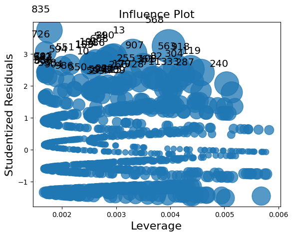
離群值和影響¶

Statsmodels 為非線性模型（具有非線性期望均值的模型）提供了一個通用的 MLEInfluence 類別，適用於離散模型和其他基於最大概似法的模型，例如 Beta 迴歸模型。提供的度量基於一般定義，例如廣義槓桿而不是線性模型中的帽子矩陣的對角線。

結果方法 get_influence 回傳 MLEInfluence 類別的實例，該實例具有各種離群值和影響度量的方法。

[33]:

infl = res.get_influence()
[i for i in dir(infl) if not i.startswith("_")]

[33]:

['cooks_distance',
 'cov_params',
 'd_fittedvalues',
 'd_fittedvalues_scaled',
 'd_params',
 'dfbetas',
 'endog',
 'exog',
 'hat_matrix_diag',
 'hat_matrix_exog_diag',
 'hessian',
 'k_params',
 'k_vars',
 'model_class',
 'nobs',
 'params_one',
 'plot_index',
 'plot_influence',
 'resid',
 'resid_score',
 'resid_score_factor',
 'resid_studentized',
 'results',
 'scale',
 'score_obs',
 'summary_frame']

影響類別有兩個繪圖方法。但是，由於樣本數較大，因此在這種情況下，繪圖過於擁擠。

[34]:

infl.plot_influence();

../../../_images/examples_notebooks_generated_postestimation_poisson_55_0.png

[35]:

infl.plot_index(y_var="resid_studentized");

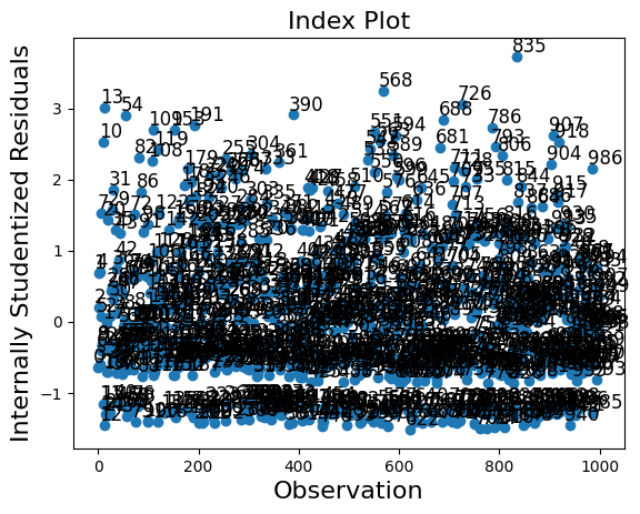
../../../_images/examples_notebooks_generated_postestimation_poisson_56_0.png

summary_frame 顯示每個觀察值的主要影響和離群值度量。

在我們的範例中，我們有 1000 個觀察值，這太多而無法輕易顯示。我們可以按其中一個列對摘要資料框架進行排序，並列出具有最大離群值或影響度量的觀察值。在下面的範例中，我們按庫克距離和 standard_resid（在一般情況下是皮爾森殘差）排序。

由於我們模擬了一個「好的」模型，因此沒有具有較大影響或較大離群值的觀察值。

[36]:

df_infl = infl.summary_frame()
df_infl.head()

[36]:

	dfb_x1	dfb_x2	dfb_x3	cooks_d	standard_resid	hat_diag	dffits_internal
0	-0.010856	0.011384	-0.013643	0.000440	-0.636944	0.003243	-0.036334
1	0.001990	-0.023625	0.028313	0.000737	0.680823	0.004749	0.047031
2	0.005794	-0.000787	0.000943	0.000035	0.201681	0.002607	0.010311
3	-0.014243	0.005539	-0.006639	0.000325	-0.589923	0.002790	-0.031206
4	0.003602	-0.022549	0.027024	0.000738	0.702888	0.004462	0.047057

[37]:

df_infl.sort_values("cooks_d", ascending=False)[:10]

[37]:

	dfb_x1	dfb_x2	dfb_x3	cooks_d	standard_resid	hat_diag	dffits_internal
568	-0.110520	-0.038997	0.143106	0.013922	3.236167	0.003972	0.204365
13	0.048914	-0.056713	0.067969	0.010034	3.011778	0.003307	0.173497
918	-0.093971	-0.038431	0.121677	0.009304	2.519367	0.004378	0.167066
563	-0.089917	-0.033708	0.116428	0.008935	2.545624	0.004119	0.163720
119	0.163230	0.103957	-0.124589	0.008883	2.409646	0.004569	0.163247
390	0.148697	0.066972	-0.080264	0.008358	2.907190	0.002958	0.158345
835	-0.017672	0.066475	0.022883	0.008209	3.727645	0.001769	0.156931
54	0.145944	0.064216	-0.076961	0.008156	2.892554	0.002916	0.156419
907	-0.078901	-0.020908	0.102164	0.008021	2.615676	0.003505	0.155126
304	0.152905	0.093680	-0.112272	0.007821	2.351520	0.004225	0.153179

[38]:

df_infl.sort_values("standard_resid", ascending=False)[:10]

[38]:

	dfb_x1	dfb_x2	dfb_x3	cooks_d	standard_resid	hat_diag	dffits_internal
835	-0.017672	0.066475	0.022883	0.008209	3.727645	0.001769	0.156931
568	-0.110520	-0.038997	0.143106	0.013922	3.236167	0.003972	0.204365
726	-0.003941	0.065200	0.005103	0.005303	3.056406	0.001700	0.126127
13	0.048914	-0.056713	0.067969	0.010034	3.011778	0.003307	0.173497
390	0.148697	0.066972	-0.080264	0.008358	2.907190	0.002958	0.158345
54	0.145944	0.064216	-0.076961	0.008156	2.892554	0.002916	0.156419
688	0.083205	0.148254	-0.107737	0.007606	2.833988	0.002833	0.151057
191	0.122062	0.040388	-0.048403	0.006704	2.764369	0.002625	0.141815
786	-0.061179	-0.000408	0.079217	0.006827	2.724900	0.002751	0.143110
109	0.110999	0.029401	-0.035236	0.006212	2.704144	0.002542	0.136518

上次更新：2024 年 10 月 03 日