離散選擇模型
Fair 的婚外情數據
紅皮書在 1974 年對女性進行了一項調查,詢問婚外情。
[1]:
%matplotlib inline
[2]:
import matplotlib.pyplot as plt
import numpy as np
import pandas as pd
import statsmodels.api as sm
from scipy import stats
from statsmodels.formula.api import logit
[3]:
print(sm.datasets.fair.SOURCE)
Fair, Ray. 1978. "A Theory of Extramarital Affairs," `Journal of Political
Economy`, February, 45-61.

The data is available at http://fairmodel.econ.yale.edu/rayfair/pdf/2011b.htm
[4]:
print(sm.datasets.fair.NOTE)
::

    Number of observations: 6366
    Number of variables: 9
    Variable name definitions:

        rate_marriage   : How rate marriage, 1 = very poor, 2 = poor, 3 = fair,
                        4 = good, 5 = very good
        age             : Age
        yrs_married     : No. years married. Interval approximations. See
                        original paper for detailed explanation.
        children        : No. children
        religious       : How relgious, 1 = not, 2 = mildly, 3 = fairly,
                        4 = strongly
        educ            : Level of education, 9 = grade school, 12 = high
                        school, 14 = some college, 16 = college graduate,
                        17 = some graduate school, 20 = advanced degree
        occupation      : 1 = student, 2 = farming, agriculture; semi-skilled,
                        or unskilled worker; 3 = white-colloar; 4 = teacher
                        counselor social worker, nurse; artist, writers;
                        technician, skilled worker, 5 = managerial,
                        administrative, business, 6 = professional with
                        advanced degree
        occupation_husb : Husband's occupation. Same as occupation.
        affairs         : measure of time spent in extramarital affairs

    See the original paper for more details.
[5]:
dta = sm.datasets.fair.load_pandas().data
[6]:
dta["affair"] = (dta["affairs"] > 0).astype(float)
print(dta.head(10))
   rate_marriage   age  yrs_married  children  religious  educ  occupation  \
0            3.0  32.0          9.0       3.0        3.0  17.0         2.0
1            3.0  27.0         13.0       3.0        1.0  14.0         3.0
2            4.0  22.0          2.5       0.0        1.0  16.0         3.0
3            4.0  37.0         16.5       4.0        3.0  16.0         5.0
4            5.0  27.0          9.0       1.0        1.0  14.0         3.0
5            4.0  27.0          9.0       0.0        2.0  14.0         3.0
6            5.0  37.0         23.0       5.5        2.0  12.0         5.0
7            5.0  37.0         23.0       5.5        2.0  12.0         2.0
8            3.0  22.0          2.5       0.0        2.0  12.0         3.0
9            3.0  27.0          6.0       0.0        1.0  16.0         3.0

   occupation_husb   affairs  affair
0              5.0  0.111111     1.0
1              4.0  3.230769     1.0
2              5.0  1.400000     1.0
3              5.0  0.727273     1.0
4              4.0  4.666666     1.0
5              4.0  4.666666     1.0
6              4.0  0.852174     1.0
7              3.0  1.826086     1.0
8              3.0  4.799999     1.0
9              5.0  1.333333     1.0
[7]:
print(dta.describe())
       rate_marriage          age  yrs_married     children    religious  \
count    6366.000000  6366.000000  6366.000000  6366.000000  6366.000000
mean        4.109645    29.082862     9.009425     1.396874     2.426170
std         0.961430     6.847882     7.280120     1.433471     0.878369
min         1.000000    17.500000     0.500000     0.000000     1.000000
25%         4.000000    22.000000     2.500000     0.000000     2.000000
50%         4.000000    27.000000     6.000000     1.000000     2.000000
75%         5.000000    32.000000    16.500000     2.000000     3.000000
max         5.000000    42.000000    23.000000     5.500000     4.000000

              educ   occupation  occupation_husb      affairs       affair
count  6366.000000  6366.000000      6366.000000  6366.000000  6366.000000
mean     14.209865     3.424128         3.850141     0.705374     0.322495
std       2.178003     0.942399         1.346435     2.203374     0.467468
min       9.000000     1.000000         1.000000     0.000000     0.000000
25%      12.000000     3.000000         3.000000     0.000000     0.000000
50%      14.000000     3.000000         4.000000     0.000000     0.000000
75%      16.000000     4.000000         5.000000     0.484848     1.000000
max      20.000000     6.000000         6.000000    57.599991     1.000000
[8]:
affair_mod = logit(
    "affair ~ occupation + educ + occupation_husb"
    "+ rate_marriage + age + yrs_married + children"
    " + religious",
    dta,
).fit()
Optimization terminated successfully.
         Current function value: 0.545314
         Iterations 6
[9]:
print(affair_mod.summary())
                           Logit Regression Results
==============================================================================
Dep. Variable:                 affair   No. Observations:                 6366
Model:                          Logit   Df Residuals:                     6357
Method:                           MLE   Df Model:                            8
Date:                Thu, 03 Oct 2024   Pseudo R-squ.:                  0.1327
Time:                        15:44:50   Log-Likelihood:                -3471.5
converged:                       True   LL-Null:                       -4002.5
Covariance Type:            nonrobust   LLR p-value:                5.807e-224
===================================================================================
                      coef    std err          z      P>|z|      [0.025      0.975]
-----------------------------------------------------------------------------------
Intercept           3.7257      0.299     12.470      0.000       3.140       4.311
occupation          0.1602      0.034      4.717      0.000       0.094       0.227
educ               -0.0392      0.015     -2.533      0.011      -0.070      -0.009
occupation_husb     0.0124      0.023      0.541      0.589      -0.033       0.057
rate_marriage      -0.7161      0.031    -22.784      0.000      -0.778      -0.655
age                -0.0605      0.010     -5.885      0.000      -0.081      -0.040
yrs_married         0.1100      0.011     10.054      0.000       0.089       0.131
children           -0.0042      0.032     -0.134      0.893      -0.066       0.058
religious          -0.3752      0.035    -10.792      0.000      -0.443      -0.307
===================================================================================
我們的預測效果如何?
[10]:
affair_mod.pred_table()
[10]:
array([[3882.,  431.],
       [1326.,  727.]])
離散選擇模型的係數並沒有告訴我們太多。我們想要的是邊際效應。
[11]:
mfx = affair_mod.get_margeff()
print(mfx.summary())
        Logit Marginal Effects
=====================================
Dep. Variable:                 affair
Method:                          dydx
At:                           overall
===================================================================================
                     dy/dx    std err          z      P>|z|      [0.025      0.975]
-----------------------------------------------------------------------------------
occupation          0.0293      0.006      4.744      0.000       0.017       0.041
educ               -0.0072      0.003     -2.538      0.011      -0.013      -0.002
occupation_husb     0.0023      0.004      0.541      0.589      -0.006       0.010
rate_marriage      -0.1308      0.005    -26.891      0.000      -0.140      -0.121
age                -0.0110      0.002     -5.937      0.000      -0.015      -0.007
yrs_married         0.0201      0.002     10.327      0.000       0.016       0.024
children           -0.0008      0.006     -0.134      0.893      -0.012       0.011
religious          -0.0685      0.006    -11.119      0.000      -0.081      -0.056
===================================================================================
[12]:
respondent1000 = dta.iloc[1000]
print(respondent1000)
rate_marriage       4.000000
age                37.000000
yrs_married        23.000000
children            3.000000
religious           3.000000
educ               12.000000
occupation          3.000000
occupation_husb     4.000000
affairs             0.521739
affair              1.000000
Name: 1000, dtype: float64
[13]:
resp = dict(
    zip(
        range(1, 9),
        respondent1000[
            [
                "occupation",
                "educ",
                "occupation_husb",
                "rate_marriage",
                "age",
                "yrs_married",
                "children",
                "religious",
            ]
        ].tolist(),
    )
)
resp.update({0: 1})
print(resp)
{1: 3.0, 2: 12.0, 3: 4.0, 4: 4.0, 5: 37.0, 6: 23.0, 7: 3.0, 8: 3.0, 0: 1}
[14]:
mfx = affair_mod.get_margeff(atexog=resp)
print(mfx.summary())
        Logit Marginal Effects
=====================================
Dep. Variable:                 affair
Method:                          dydx
At:                           overall
===================================================================================
                     dy/dx    std err          z      P>|z|      [0.025      0.975]
-----------------------------------------------------------------------------------
occupation          0.0400      0.008      4.711      0.000       0.023       0.057
educ               -0.0098      0.004     -2.537      0.011      -0.017      -0.002
occupation_husb     0.0031      0.006      0.541      0.589      -0.008       0.014
rate_marriage      -0.1788      0.008    -22.743      0.000      -0.194      -0.163
age                -0.0151      0.003     -5.928      0.000      -0.020      -0.010
yrs_married         0.0275      0.003     10.256      0.000       0.022       0.033
children           -0.0011      0.008     -0.134      0.893      -0.017       0.014
religious          -0.0937      0.009    -10.722      0.000      -0.111      -0.077
===================================================================================
predict 期望一個 DataFrame,因為 patsy 用於選擇欄位。
[15]:
respondent1000 = dta.iloc[[1000]]
affair_mod.predict(respondent1000)
[15]:
1000    0.518782
dtype: float64
[16]:
affair_mod.fittedvalues[1000]
[16]:
np.float64(0.0751615928505458)
[17]:
affair_mod.model.cdf(affair_mod.fittedvalues[1000])
[17]:
np.float64(0.5187815572121427)
這裡「正確」的模型很可能是 Tobit 模型。如果有人對審查迴歸模型感興趣,我們在 github 上有一個正在進行中的分支「tobit-model」。
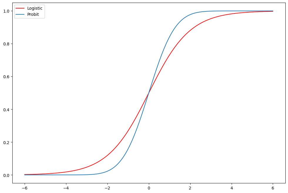
練習:羅吉斯 vs 普羅比
[18]:
fig = plt.figure(figsize=(12, 8))
ax = fig.add_subplot(111)
support = np.linspace(-6, 6, 1000)
ax.plot(support, stats.logistic.cdf(support), "r-", label="Logistic")
ax.plot(support, stats.norm.cdf(support), label="Probit")
ax.legend()
[18]:
<matplotlib.legend.Legend at 0x7fcf30701ff0>
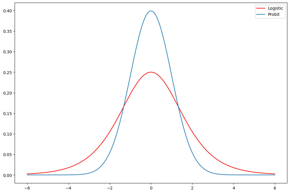
[19]:
fig = plt.figure(figsize=(12, 8))
ax = fig.add_subplot(111)
support = np.linspace(-6, 6, 1000)
ax.plot(support, stats.logistic.pdf(support), "r-", label="Logistic")
ax.plot(support, stats.norm.pdf(support), label="Probit")
ax.legend()
[19]:
<matplotlib.legend.Legend at 0x7fcf3061e410>
將上述羅吉斯 Fair 模型的估計值與普羅比模型進行比較。預測表看起來更好嗎?邊際效應有很大的差異嗎?
廣義線性模型範例
[20]:
print(sm.datasets.star98.SOURCE)
Jeff Gill's `Generalized Linear Models: A Unified Approach`

http://jgill.wustl.edu/research/books.html
[21]:
print(sm.datasets.star98.DESCRLONG)
This data is on the California education policy and outcomes (STAR program
results for 1998.  The data measured standardized testing by the California
Department of Education that required evaluation of 2nd - 11th grade students
by the the Stanford 9 test on a variety of subjects.  This dataset is at
the level of the unified school district and consists of 303 cases.  The
binary response variable represents the number of 9th graders scoring
over the national median value on the mathematics exam.

The data used in this example is only a subset of the original source.
[22]:
print(sm.datasets.star98.NOTE)
::

    Number of Observations - 303 (counties in California).

    Number of Variables - 13 and 8 interaction terms.

    Definition of variables names::

        NABOVE   - Total number of students above the national median for the
                   math section.
        NBELOW   - Total number of students below the national median for the
                   math section.
        LOWINC   - Percentage of low income students
        PERASIAN - Percentage of Asian student
        PERBLACK - Percentage of black students
        PERHISP  - Percentage of Hispanic students
        PERMINTE - Percentage of minority teachers
        AVYRSEXP - Sum of teachers' years in educational service divided by the
                number of teachers.
        AVSALK   - Total salary budget including benefits divided by the number
                   of full-time teachers (in thousands)
        PERSPENK - Per-pupil spending (in thousands)
        PTRATIO  - Pupil-teacher ratio.
        PCTAF    - Percentage of students taking UC/CSU prep courses
        PCTCHRT  - Percentage of charter schools
        PCTYRRND - Percentage of year-round schools

        The below variables are interaction terms of the variables defined
        above.

        PERMINTE_AVYRSEXP
        PEMINTE_AVSAL
        AVYRSEXP_AVSAL
        PERSPEN_PTRATIO
        PERSPEN_PCTAF
        PTRATIO_PCTAF
        PERMINTE_AVTRSEXP_AVSAL
        PERSPEN_PTRATIO_PCTAF
[23]:
dta = sm.datasets.star98.load_pandas().data
print(dta.columns)
Index(['NABOVE', 'NBELOW', 'LOWINC', 'PERASIAN', 'PERBLACK', 'PERHISP',
       'PERMINTE', 'AVYRSEXP', 'AVSALK', 'PERSPENK', 'PTRATIO', 'PCTAF',
       'PCTCHRT', 'PCTYRRND', 'PERMINTE_AVYRSEXP', 'PERMINTE_AVSAL',
       'AVYRSEXP_AVSAL', 'PERSPEN_PTRATIO', 'PERSPEN_PCTAF', 'PTRATIO_PCTAF',
       'PERMINTE_AVYRSEXP_AVSAL', 'PERSPEN_PTRATIO_PCTAF'],
      dtype='object')
[24]:
print(
    dta[
        ["NABOVE", "NBELOW", "LOWINC", "PERASIAN", "PERBLACK", "PERHISP", "PERMINTE"]
    ].head(10)
)
   NABOVE  NBELOW    LOWINC   PERASIAN   PERBLACK    PERHISP   PERMINTE
0   452.0   355.0  34.39730  23.299300  14.235280  11.411120  15.918370
1   144.0    40.0  17.36507  29.328380   8.234897   9.314884  13.636360
2   337.0   234.0  32.64324   9.226386  42.406310  13.543720  28.834360
3   395.0   178.0  11.90953  13.883090   3.796973  11.443110  11.111110
4     8.0    57.0  36.88889  12.187500  76.875000   7.604167  43.589740
5  1348.0   899.0  20.93149  28.023510   4.643221  13.808160  15.378490
6   477.0   887.0  53.26898   8.447858  19.374830  37.905330  25.525530
7   565.0   347.0  15.19009   3.665781   2.649680  13.092070   6.203008
8   205.0   320.0  28.21582  10.430420   6.786374  32.334300  13.461540
9   469.0   598.0  32.77897  17.178310  12.484930  28.323290  27.259890
[25]:
print(
    dta[
        ["AVYRSEXP", "AVSALK", "PERSPENK", "PTRATIO", "PCTAF", "PCTCHRT", "PCTYRRND"]
    ].head(10)
)
   AVYRSEXP    AVSALK  PERSPENK   PTRATIO     PCTAF  PCTCHRT   PCTYRRND
0  14.70646  59.15732  4.445207  21.71025  57.03276      0.0  22.222220
1  16.08324  59.50397  5.267598  20.44278  64.62264      0.0   0.000000
2  14.59559  60.56992  5.482922  18.95419  53.94191      0.0   0.000000
3  14.38939  58.33411  4.165093  21.63539  49.06103      0.0   7.142857
4  13.90568  63.15364  4.324902  18.77984  52.38095      0.0   0.000000
5  14.97755  66.97055  3.916104  24.51914  44.91578      0.0   2.380952
6  14.67829  57.62195  4.270903  22.21278  32.28916      0.0  12.121210
7  13.66197  63.44740  4.309734  24.59026  30.45267      0.0   0.000000
8  16.41760  57.84564  4.527603  21.74138  22.64574      0.0   0.000000
9  12.51864  57.80141  4.648917  20.26010  26.07099      0.0   0.000000
[26]:
formula = "NABOVE + NBELOW ~ LOWINC + PERASIAN + PERBLACK + PERHISP + PCTCHRT "
formula += "+ PCTYRRND + PERMINTE*AVYRSEXP*AVSALK + PERSPENK*PTRATIO*PCTAF"
旁註:二項分佈
擲一個六面骰子 5 次,剛好出現 2 個 4 的機率是多少?
[27]:
stats.binom(5, 1.0 / 6).pmf(2)
[27]:
np.float64(0.16075102880658423)
[28]:
from scipy.special import comb

comb(5, 2) * (1 / 6.0) ** 2 * (5 / 6.0) ** 3
[28]:
np.float64(0.1607510288065844)
[29]:
from statsmodels.formula.api import glm

glm_mod = glm(formula, dta, family=sm.families.Binomial()).fit()
[30]:
print(glm_mod.summary())
                  Generalized Linear Model Regression Results
================================================================================
Dep. Variable:     ['NABOVE', 'NBELOW']   No. Observations:                  303
Model:                              GLM   Df Residuals:                      282
Model Family:                  Binomial   Df Model:                           20
Link Function:                    Logit   Scale:                          1.0000
Method:                            IRLS   Log-Likelihood:                -2998.6
Date:                  Thu, 03 Oct 2024   Deviance:                       4078.8
Time:                          15:44:51   Pearson chi2:                 4.05e+03
No. Iterations:                       5   Pseudo R-squ. (CS):              1.000
Covariance Type:              nonrobust
============================================================================================
                               coef    std err          z      P>|z|      [0.025      0.975]
--------------------------------------------------------------------------------------------
Intercept                    2.9589      1.547      1.913      0.056      -0.073       5.990
LOWINC                      -0.0168      0.000    -38.749      0.000      -0.018      -0.016
PERASIAN                     0.0099      0.001     16.505      0.000       0.009       0.011
PERBLACK                    -0.0187      0.001    -25.182      0.000      -0.020      -0.017
PERHISP                     -0.0142      0.000    -32.818      0.000      -0.015      -0.013
PCTCHRT                      0.0049      0.001      3.921      0.000       0.002       0.007
PCTYRRND                    -0.0036      0.000    -15.878      0.000      -0.004      -0.003
PERMINTE                     0.2545      0.030      8.498      0.000       0.196       0.313
AVYRSEXP                     0.2407      0.057      4.212      0.000       0.129       0.353
PERMINTE:AVYRSEXP           -0.0141      0.002     -7.391      0.000      -0.018      -0.010
AVSALK                       0.0804      0.014      5.775      0.000       0.053       0.108
PERMINTE:AVSALK             -0.0040      0.000     -8.450      0.000      -0.005      -0.003
AVYRSEXP:AVSALK             -0.0039      0.001     -4.059      0.000      -0.006      -0.002
PERMINTE:AVYRSEXP:AVSALK     0.0002   2.99e-05      7.428      0.000       0.000       0.000
PERSPENK                    -1.9522      0.317     -6.162      0.000      -2.573      -1.331
PTRATIO                     -0.3341      0.061     -5.453      0.000      -0.454      -0.214
PERSPENK:PTRATIO             0.0917      0.015      6.321      0.000       0.063       0.120
PCTAF                       -0.1690      0.033     -5.169      0.000      -0.233      -0.105
PERSPENK:PCTAF               0.0490      0.007      6.574      0.000       0.034       0.064
PTRATIO:PCTAF                0.0080      0.001      5.362      0.000       0.005       0.011
PERSPENK:PTRATIO:PCTAF      -0.0022      0.000     -6.445      0.000      -0.003      -0.002
============================================================================================
試驗次數
[31]:
glm_mod.model.data.orig_endog.sum(1)
[31]:
0      807.0
1      184.0
2      571.0
3      573.0
4       65.0
       ...
298    342.0
299    154.0
300    595.0
301    709.0
302    156.0
Length: 303, dtype: float64
[32]:
glm_mod.fittedvalues * glm_mod.model.data.orig_endog.sum(1)
[32]:
0      470.732584
1      138.266178
2      285.832629
3      392.702917
4       20.963146
          ...
298    111.464708
299     61.037884
300    235.517446
301    290.952508
302     53.312851
Length: 303, dtype: float64
一階差分:我們將所有解釋變數固定在其平均值,並操縱低收入家庭的比例,以評估其對反應變數的影響
[33]:
exog = glm_mod.model.data.orig_exog # get the dataframe
[34]:
means25 = exog.mean()
print(means25)
Intercept                       1.000000
LOWINC                         41.409877
PERASIAN                        5.896335
PERBLACK                        5.636808
PERHISP                        34.398080
PCTCHRT                         1.175909
PCTYRRND                       11.611905
PERMINTE                       14.694747
AVYRSEXP                       14.253875
PERMINTE:AVYRSEXP             209.018700
AVSALK                         58.640258
PERMINTE:AVSALK               879.979883
AVYRSEXP:AVSALK               839.718173
PERMINTE:AVYRSEXP:AVSALK    12585.266464
PERSPENK                        4.320310
PTRATIO                        22.464250
PERSPENK:PTRATIO               96.295756
PCTAF                          33.630593
PERSPENK:PCTAF                147.235740
PTRATIO:PCTAF                 747.445536
PERSPENK:PTRATIO:PCTAF       3243.607568
dtype: float64
[35]:
means25["LOWINC"] = exog["LOWINC"].quantile(0.25)
print(means25)
Intercept                       1.000000
LOWINC                         26.683040
PERASIAN                        5.896335
PERBLACK                        5.636808
PERHISP                        34.398080
PCTCHRT                         1.175909
PCTYRRND                       11.611905
PERMINTE                       14.694747
AVYRSEXP                       14.253875
PERMINTE:AVYRSEXP             209.018700
AVSALK                         58.640258
PERMINTE:AVSALK               879.979883
AVYRSEXP:AVSALK               839.718173
PERMINTE:AVYRSEXP:AVSALK    12585.266464
PERSPENK                        4.320310
PTRATIO                        22.464250
PERSPENK:PTRATIO               96.295756
PCTAF                          33.630593
PERSPENK:PCTAF                147.235740
PTRATIO:PCTAF                 747.445536
PERSPENK:PTRATIO:PCTAF       3243.607568
dtype: float64
[36]:
means75 = exog.mean()
means75["LOWINC"] = exog["LOWINC"].quantile(0.75)
print(means75)
Intercept                       1.000000
LOWINC                         55.460075
PERASIAN                        5.896335
PERBLACK                        5.636808
PERHISP                        34.398080
PCTCHRT                         1.175909
PCTYRRND                       11.611905
PERMINTE                       14.694747
AVYRSEXP                       14.253875
PERMINTE:AVYRSEXP             209.018700
AVSALK                         58.640258
PERMINTE:AVSALK               879.979883
AVYRSEXP:AVSALK               839.718173
PERMINTE:AVYRSEXP:AVSALK    12585.266464
PERSPENK                        4.320310
PTRATIO                        22.464250
PERSPENK:PTRATIO               96.295756
PCTAF                          33.630593
PERSPENK:PCTAF                147.235740
PTRATIO:PCTAF                 747.445536
PERSPENK:PTRATIO:PCTAF       3243.607568
dtype: float64
同樣,predict 期望一個 DataFrame,因為 patsy 用於選擇欄位。
[37]:
resp25 = glm_mod.predict(pd.DataFrame(means25).T)
resp75 = glm_mod.predict(pd.DataFrame(means75).T)
diff = resp75 - resp25
學區中低收入家庭比例的四分位數一階差分是
[38]:
print("%2.4f%%" % (diff[0] * 100))
-11.8863%
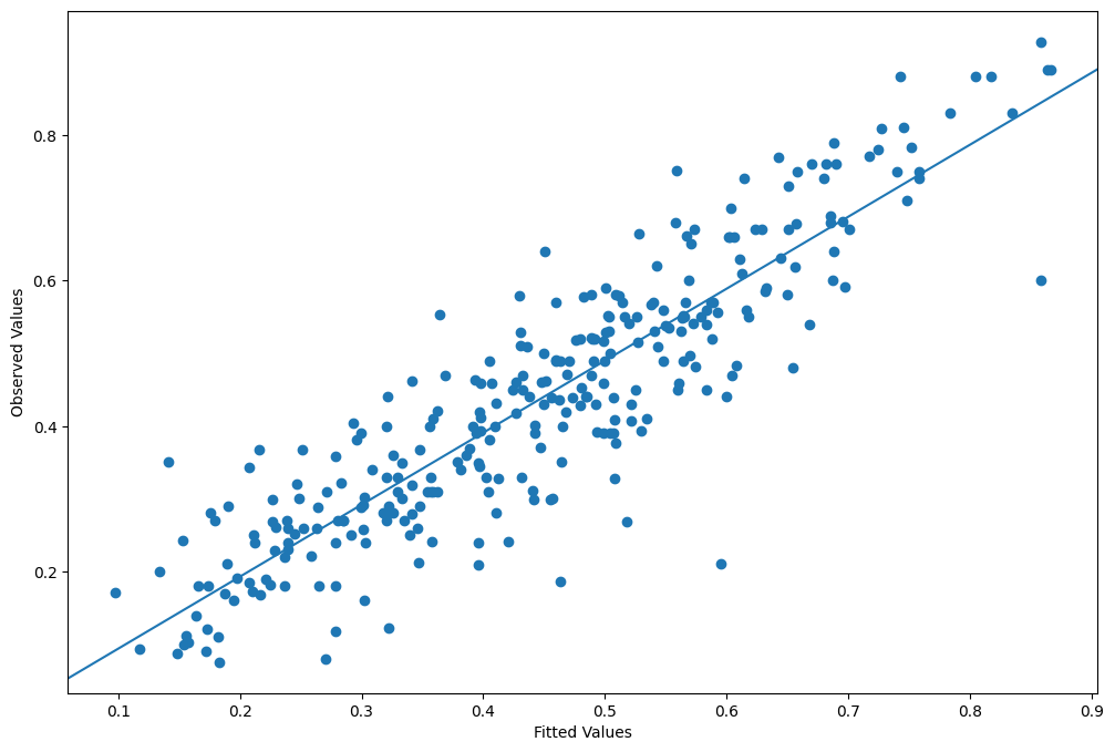
[39]:
nobs = glm_mod.nobs
y = glm_mod.model.endog
yhat = glm_mod.mu
[40]:
from statsmodels.graphics.api import abline_plot

fig = plt.figure(figsize=(12, 8))
ax = fig.add_subplot(111, ylabel="Observed Values", xlabel="Fitted Values")
ax.scatter(yhat, y)
y_vs_yhat = sm.OLS(y, sm.add_constant(yhat, prepend=True)).fit()
fig = abline_plot(model_results=y_vs_yhat, ax=ax)
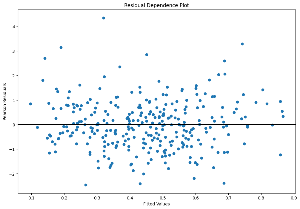
繪製擬合值 vs 皮爾森殘差
皮爾森殘差定義為
\[\frac{(y - \mu)}{\sqrt{(var(\mu))}}\]
其中 var 通常由族系決定。例如,二項式變異數為 \(np(1 - p)\)
[41]:
fig = plt.figure(figsize=(12, 8))
ax = fig.add_subplot(
    111,
    title="Residual Dependence Plot",
    xlabel="Fitted Values",
    ylabel="Pearson Residuals",
)
ax.scatter(yhat, stats.zscore(glm_mod.resid_pearson))
ax.axis("tight")
ax.plot([0.0, 1.0], [0.0, 0.0], "k-")
[41]:
[<matplotlib.lines.Line2D at 0x7fcf305d8a90>]
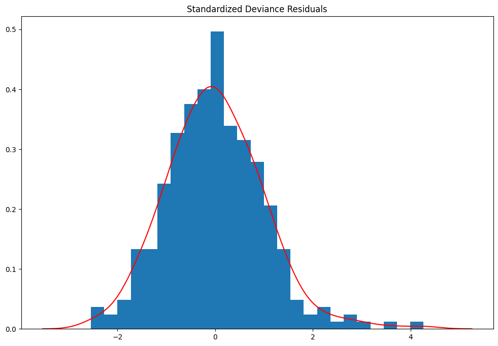
標準化離差殘差的直方圖,並覆蓋核密度估計
離差殘差的定義取決於族系。對於二項分佈,這是
\[r_{dev} = sign\left(Y-\mu\right)*\sqrt{2n(Y\log\frac{Y}{\mu}+(1-Y)\log\frac{(1-Y)}{(1-\mu)}}\]
它們可用於檢測不適當的共變量
[42]:
resid = glm_mod.resid_deviance
resid_std = stats.zscore(resid)
kde_resid = sm.nonparametric.KDEUnivariate(resid_std)
kde_resid.fit()
[42]:
<statsmodels.nonparametric.kde.KDEUnivariate at 0x7fcf304120e0>
[43]:
fig = plt.figure(figsize=(12, 8))
ax = fig.add_subplot(111, title="Standardized Deviance Residuals")
ax.hist(resid_std, bins=25, density=True)
ax.plot(kde_resid.support, kde_resid.density, "r")
[43]:
[<matplotlib.lines.Line2D at 0x7fcf3045c850>]
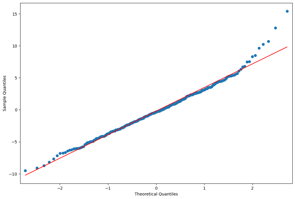
離差殘差的 QQ 圖
[44]:
fig = plt.figure(figsize=(12, 8))
ax = fig.add_subplot(111)
fig = sm.graphics.qqplot(resid, line="r", ax=ax)
上次更新:2024 年 10 月 03 日