預測(樣本外)
[1]:
%matplotlib inline
[2]:
import numpy as np
import matplotlib.pyplot as plt

import statsmodels.api as sm

plt.rc("figure", figsize=(16, 8))
plt.rc("font", size=14)
人工數據
[3]:
nsample = 50
sig = 0.25
x1 = np.linspace(0, 20, nsample)
X = np.column_stack((x1, np.sin(x1), (x1 - 5) ** 2))
X = sm.add_constant(X)
beta = [5.0, 0.5, 0.5, -0.02]
y_true = np.dot(X, beta)
y = y_true + sig * np.random.normal(size=nsample)
估計
[4]:
olsmod = sm.OLS(y, X)
olsres = olsmod.fit()
print(olsres.summary())
                            OLS Regression Results
==============================================================================
Dep. Variable:                      y   R-squared:                       0.980
Model:                            OLS   Adj. R-squared:                  0.979
Method:                 Least Squares   F-statistic:                     767.8
Date:                Thu, 03 Oct 2024   Prob (F-statistic):           2.80e-39
Time:                        15:50:37   Log-Likelihood:                -3.6609
No. Observations:                  50   AIC:                             15.32
Df Residuals:                      46   BIC:                             22.97
Df Model:                           3
Covariance Type:            nonrobust
==============================================================================
                 coef    std err          t      P>|t|      [0.025      0.975]
------------------------------------------------------------------------------
const          5.0304      0.093     54.373      0.000       4.844       5.217
x1             0.5002      0.014     35.058      0.000       0.471       0.529
x2             0.5011      0.056      8.934      0.000       0.388       0.614
x3            -0.0201      0.001    -16.012      0.000      -0.023      -0.018
==============================================================================
Omnibus:                        2.155   Durbin-Watson:                   1.847
Prob(Omnibus):                  0.340   Jarque-Bera (JB):                2.068
Skew:                          -0.462   Prob(JB):                        0.356
Kurtosis:                       2.630   Cond. No.                         221.
==============================================================================

Notes:
[1] Standard Errors assume that the covariance matrix of the errors is correctly specified.
樣本內預測
[5]:
ypred = olsres.predict(X)
print(ypred)
[ 4.52892208  5.01052175  5.45275967  5.82832671  6.11976948  6.32235784
  6.44486207  6.50811191  6.54157432  6.57851213  6.65051904  6.7823289
  6.98775197  7.26740594  7.60861448  7.98748987  8.37285773  8.73137887
  9.03302681  9.25602105  9.39040558  9.43968456  9.42024665  9.35867239
  9.28736706  9.23923662  9.24228135  9.31499546  9.46332857  9.67970819
  9.94428385 10.2281885  10.49828128 10.72259244 10.87557591 10.94230645
 10.9209318  10.82297701 10.67145093 10.49706588 10.33319174 10.21037335
 10.15131209 10.1671361  10.25557197 10.40131825 10.57855941 10.75520731
 10.89817315 10.97880387]
建立新的解釋變數 Xnew 樣本,進行預測並繪圖
[6]:
x1n = np.linspace(20.5, 25, 10)
Xnew = np.column_stack((x1n, np.sin(x1n), (x1n - 5) ** 2))
Xnew = sm.add_constant(Xnew)
ynewpred = olsres.predict(Xnew)  # predict out of sample
print(ynewpred)
[10.96503747 10.81894524 10.56017815 10.23351824  9.89791447  9.61204991
  9.4199741   9.34031818  9.36173334  9.44566941]
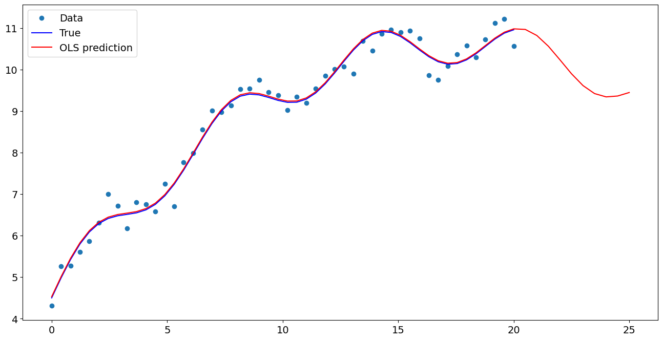
繪圖比較
[7]:
import matplotlib.pyplot as plt

fig, ax = plt.subplots()
ax.plot(x1, y, "o", label="Data")
ax.plot(x1, y_true, "b-", label="True")
ax.plot(np.hstack((x1, x1n)), np.hstack((ypred, ynewpred)), "r", label="OLS prediction")
ax.legend(loc="best")
[7]:
<matplotlib.legend.Legend at 0x7f30514b3fd0>
使用公式進行預測
使用公式可以讓估計和預測變得更容易
[8]:
from statsmodels.formula.api import ols

data = {"x1": x1, "y": y}

res = ols("y ~ x1 + np.sin(x1) + I((x1-5)**2)", data=data).fit()
我們使用 I 來表示使用恆等變換。也就是說,我們不希望使用 **2 進行任何擴展
[9]:
res.params
[9]:
Intercept           5.030411
x1                  0.500216
np.sin(x1)          0.501093
I((x1 - 5) ** 2)   -0.020060
dtype: float64
現在我們只需要傳遞單個變數,就可以自動獲得轉換後的右側變數
[10]:
res.predict(exog=dict(x1=x1n))
[10]:
0    10.965037
1    10.818945
2    10.560178
3    10.233518
4     9.897914
5     9.612050
6     9.419974
7     9.340318
8     9.361733
9     9.445669
dtype: float64
上次更新:2024 年 10 月 03 日