statsmodels 中的預測
此筆記本說明如何在 statsmodels 中使用時間序列模型進行預測。
注意:此筆記本僅適用於狀態空間模型類別,這些類別為
sm.tsa.SARIMAXsm.tsa.UnobservedComponentssm.tsa.VARMAXsm.tsa.DynamicFactor
[1]:
%matplotlib inline

import numpy as np
import pandas as pd
import statsmodels.api as sm
import matplotlib.pyplot as plt

macrodata = sm.datasets.macrodata.load_pandas().data
macrodata.index = pd.period_range('1959Q1', '2009Q3', freq='Q')
基本範例
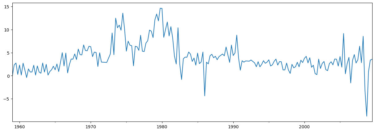
一個簡單的範例是使用 AR(1) 模型來預測通貨膨脹。在預測之前,讓我們先看看這個序列
[2]:
endog = macrodata['infl']
endog.plot(figsize=(15, 5))
[2]:
<Axes: >
建構和估計模型
下一步是制定我們要用於預測的計量經濟模型。 在此情況下,我們將透過 statsmodels 中的 SARIMAX 類別使用 AR(1) 模型。
建構模型後,我們需要估計其參數。 這可以使用 fit 方法來完成。 summary 方法會產生幾個方便的表格,顯示結果。
[3]:
# Construct the model
mod = sm.tsa.SARIMAX(endog, order=(1, 0, 0), trend='c')
# Estimate the parameters
res = mod.fit()

print(res.summary())
RUNNING THE L-BFGS-B CODE

           * * *

Machine precision = 2.220D-16
 N =            3     M =           10

At X0         0 variables are exactly at the bounds

At iterate    0    f=  2.32873D+00    |proj g|=  8.23649D-03

At iterate    5    f=  2.32864D+00    |proj g|=  1.41994D-03

           * * *

Tit   = total number of iterations
Tnf   = total number of function evaluations
Tnint = total number of segments explored during Cauchy searches
Skip  = number of BFGS updates skipped
Nact  = number of active bounds at final generalized Cauchy point
Projg = norm of the final projected gradient
F     = final function value

           * * *

   N    Tit     Tnf  Tnint  Skip  Nact     Projg        F
    3      8     10      1     0     0   5.820D-06   2.329D+00
  F =   2.3286389358138617

CONVERGENCE: NORM_OF_PROJECTED_GRADIENT_<=_PGTOL
                               SARIMAX Results
==============================================================================
Dep. Variable:                   infl   No. Observations:                  203
Model:               SARIMAX(1, 0, 0)   Log Likelihood                -472.714
Date:                Thu, 03 Oct 2024   AIC                            951.427
Time:                        16:07:30   BIC                            961.367
Sample:                    03-31-1959   HQIC                           955.449
                         - 09-30-2009
Covariance Type:                  opg
==============================================================================
                 coef    std err          z      P>|z|      [0.025      0.975]
------------------------------------------------------------------------------
intercept      1.3962      0.254      5.488      0.000       0.898       1.895
ar.L1          0.6441      0.039     16.482      0.000       0.568       0.721
sigma2         6.1519      0.397     15.487      0.000       5.373       6.930
===================================================================================
Ljung-Box (L1) (Q):                   8.43   Jarque-Bera (JB):                68.45
Prob(Q):                              0.00   Prob(JB):                         0.00
Heteroskedasticity (H):               1.47   Skew:                            -0.22
Prob(H) (two-sided):                  0.12   Kurtosis:                         5.81
===================================================================================

Warnings:
[1] Covariance matrix calculated using the outer product of gradients (complex-step).
This problem is unconstrained.
預測
樣本外預測是使用結果物件中的 forecast 或 get_forecast 方法產生的。
forecast 方法僅提供點預測。
[4]:
# The default is to get a one-step-ahead forecast:
print(res.forecast())
2009Q4    3.68921
Freq: Q-DEC, dtype: float64
get_forecast 方法更通用,也允許建構信賴區間。
[5]:
# Here we construct a more complete results object.
fcast_res1 = res.get_forecast()

# Most results are collected in the `summary_frame` attribute.
# Here we specify that we want a confidence level of 90%
print(fcast_res1.summary_frame(alpha=0.10))
infl       mean   mean_se  mean_ci_lower  mean_ci_upper
2009Q4  3.68921  2.480302      -0.390523       7.768943
預設的信賴水準為 95%,但這可以透過設定 alpha 參數來控制,其中信賴水準定義為 \((1 - \alpha) \times 100\%\)。 在上面的範例中,我們使用 alpha=0.10 指定了 90% 的信賴水準。
指定預測數量
forecast 和 get_forecast 這兩個函式都接受單一引數,指示所需的預測步驟數。 此引數的一個選項是始終提供一個整數,描述您想要向前預測的步驟數。
[6]:
print(res.forecast(steps=2))
2009Q4    3.689210
2010Q1    3.772434
Freq: Q-DEC, Name: predicted_mean, dtype: float64
[7]:
fcast_res2 = res.get_forecast(steps=2)
# Note: since we did not specify the alpha parameter, the
# confidence level is at the default, 95%
print(fcast_res2.summary_frame())
infl        mean   mean_se  mean_ci_lower  mean_ci_upper
2009Q4  3.689210  2.480302      -1.172092       8.550512
2010Q1  3.772434  2.950274      -2.009996       9.554865
但是,如果您的資料包含具有已定義頻率的 Pandas 索引(有關更多資訊,請參閱結尾的索引章節),那麼您可以選擇指定您想要產生預測的日期
[8]:
print(res.forecast('2010Q2'))
2009Q4    3.689210
2010Q1    3.772434
2010Q2    3.826039
Freq: Q-DEC, Name: predicted_mean, dtype: float64
[9]:
fcast_res3 = res.get_forecast('2010Q2')
print(fcast_res3.summary_frame())
infl        mean   mean_se  mean_ci_lower  mean_ci_upper
2009Q4  3.689210  2.480302      -1.172092       8.550512
2010Q1  3.772434  2.950274      -2.009996       9.554865
2010Q2  3.826039  3.124571      -2.298008       9.950087
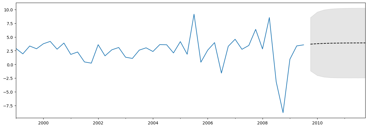
繪製資料、預測和信賴區間
通常,繪製資料、預測和信賴區間很有用。 有很多方法可以做到這一點,但這是一個範例
[10]:
fig, ax = plt.subplots(figsize=(15, 5))

# Plot the data (here we are subsetting it to get a better look at the forecasts)
endog.loc['1999':].plot(ax=ax)

# Construct the forecasts
fcast = res.get_forecast('2011Q4').summary_frame()
fcast['mean'].plot(ax=ax, style='k--')
ax.fill_between(fcast.index, fcast['mean_ci_lower'], fcast['mean_ci_upper'], color='k', alpha=0.1);
關於預測的注意事項
上面的預測可能看起來不是很令人印象深刻,因為它幾乎是一條直線。 這是因為這是一個非常簡單的單變量預測模型。 然而,請記住,這些簡單的預測模型可能非常具有競爭力。
預測 vs. 預報
結果物件還包含兩個方法,適用於樣本內擬合值和樣本外預測。 它們是 predict 和 get_prediction。predict 方法僅傳回點預測(類似於 forecast),而 get_prediction 方法也傳回額外的結果(類似於 get_forecast)。
一般而言,如果您感興趣的是樣本外預測,則堅持使用 forecast 和 get_forecast 方法會更容易。
交叉驗證
注意:本節中使用的一些函式最早在 statsmodels v0.11.0 中引入。
一個常見的用例是透過使用以下過程遞迴執行 h 步前預測來交叉驗證預測方法
在訓練樣本上擬合模型參數
從該樣本的結尾產生 h 步前預測
將預測與測試資料集進行比較以計算錯誤率
擴展樣本以包含下一個觀察值,然後重複
經濟學家有時將其稱為虛擬樣本外預測評估練習或時間序列交叉驗證。
範例
我們將使用上面的通貨膨脹資料集進行非常簡單的這種類型練習。 完整資料集包含 203 個觀察值,為了解釋起見,我們將使用前 80% 作為我們的訓練樣本,並且僅考慮一步前預測。
上述程序的單一迭代如下所示
[11]:
# Step 1: fit model parameters w/ training sample
training_obs = int(len(endog) * 0.8)

training_endog = endog[:training_obs]
training_mod = sm.tsa.SARIMAX(
    training_endog, order=(1, 0, 0), trend='c')
training_res = training_mod.fit()

# Print the estimated parameters
print(training_res.params)
RUNNING THE L-BFGS-B CODE

           * * *

Machine precision = 2.220D-16
 N =            3     M =           10

At X0         0 variables are exactly at the bounds

At iterate    0    f=  2.23132D+00    |proj g|=  1.09171D-02

At iterate    5    f=  2.23109D+00    |proj g|=  3.93608D-05

           * * *

Tit   = total number of iterations
Tnf   = total number of function evaluations
Tnint = total number of segments explored during Cauchy searches
Skip  = number of BFGS updates skipped
Nact  = number of active bounds at final generalized Cauchy point
Projg = norm of the final projected gradient
F     = final function value

           * * *

   N    Tit     Tnf  Tnint  Skip  Nact     Projg        F
    3      6      8      1     0     0   7.066D-07   2.231D+00
  F =   2.2310884444664758

CONVERGENCE: NORM_OF_PROJECTED_GRADIENT_<=_PGTOL
intercept    1.162076
ar.L1        0.724242
sigma2       5.051600
dtype: float64
This problem is unconstrained.
[12]:
# Step 2: produce one-step-ahead forecasts
fcast = training_res.forecast()

# Step 3: compute root mean square forecasting error
true = endog.reindex(fcast.index)
error = true - fcast

# Print out the results
print(pd.concat([true.rename('true'),
                 fcast.rename('forecast'),
                 error.rename('error')], axis=1))
        true  forecast    error
1999Q3  3.35   2.55262  0.79738
若要新增另一個觀察值,我們可以使用 append 或 extend 結果方法。 這兩種方法都可以產生相同的預測,但它們在可用的其他結果方面有所不同
append是更完整的方法。 它始終儲存所有訓練觀察值的結果,並且您可以選擇在給定新觀察值的情況下重新擬合模型參數(請注意,預設值是不重新擬合參數)。extend是一種較快的方法,如果訓練樣本非常大,則可能很有用。 它僅儲存新觀察值的結果,並且不允許重新擬合模型參數(即,您必須使用在上一個樣本中估計的參數)。
如果您的訓練樣本相對較小(例如,少於幾千個觀察值),或者如果您想計算最佳預測,則應使用 append 方法。 但是,如果該方法不可行(例如,因為您有非常大的訓練樣本),或者如果您可以接受略微次優的預測(因為參數估計會稍微過時),那麼您可以考慮使用 extend 方法。
使用 append 方法並重新擬合參數的第二次迭代如下所示(再次注意,append 的預設值不會重新擬合參數,但我們已使用 refit=True 引數覆寫了該預設值)
[13]:
# Step 1: append a new observation to the sample and refit the parameters
append_res = training_res.append(endog[training_obs:training_obs + 1], refit=True)

# Print the re-estimated parameters
print(append_res.params)
RUNNING THE L-BFGS-B CODE

           * * *

Machine precision = 2.220D-16
 N =            3     M =           10

At X0         0 variables are exactly at the bounds

At iterate    0    f=  2.22839D+00    |proj g|=  2.38555D-03

At iterate    5    f=  2.22838D+00    |proj g|=  9.80105D-08

           * * *

Tit   = total number of iterations
Tnf   = total number of function evaluations
Tnint = total number of segments explored during Cauchy searches
Skip  = number of BFGS updates skipped
Nact  = number of active bounds at final generalized Cauchy point
Projg = norm of the final projected gradient
F     = final function value

           * * *

   N    Tit     Tnf  Tnint  Skip  Nact     Projg        F
    3      5      8      1     0     0   9.801D-08   2.228D+00
  F =   2.2283821699856410

CONVERGENCE: NORM_OF_PROJECTED_GRADIENT_<=_PGTOL
intercept    1.171544
ar.L1        0.723152
sigma2       5.024580
dtype: float64
This problem is unconstrained.
請注意,這些估計的參數與我們最初估計的參數略有不同。 透過新的結果物件 append_res,我們可以計算從比上次呼叫更進一步的一個觀察值開始的預測
[14]:
# Step 2: produce one-step-ahead forecasts
fcast = append_res.forecast()

# Step 3: compute root mean square forecasting error
true = endog.reindex(fcast.index)
error = true - fcast

# Print out the results
print(pd.concat([true.rename('true'),
                 fcast.rename('forecast'),
                 error.rename('error')], axis=1))
        true  forecast     error
1999Q4  2.85  3.594102 -0.744102
總而言之,我們可以按如下方式執行遞迴預測評估練習
[15]:
# Setup forecasts
nforecasts = 3
forecasts = {}

# Get the number of initial training observations
nobs = len(endog)
n_init_training = int(nobs * 0.8)

# Create model for initial training sample, fit parameters
init_training_endog = endog.iloc[:n_init_training]
mod = sm.tsa.SARIMAX(training_endog, order=(1, 0, 0), trend='c')
res = mod.fit()

# Save initial forecast
forecasts[training_endog.index[-1]] = res.forecast(steps=nforecasts)

# Step through the rest of the sample
for t in range(n_init_training, nobs):
    # Update the results by appending the next observation
    updated_endog = endog.iloc[t:t+1]
    res = res.append(updated_endog, refit=False)

    # Save the new set of forecasts
    forecasts[updated_endog.index[0]] = res.forecast(steps=nforecasts)

# Combine all forecasts into a dataframe
forecasts = pd.concat(forecasts, axis=1)

print(forecasts.iloc[:5, :5])
RUNNING THE L-BFGS-B CODE

           * * *

Machine precision = 2.220D-16
 N =            3     M =           10

At X0         0 variables are exactly at the bounds

At iterate    0    f=  2.23132D+00    |proj g|=  1.09171D-02
This problem is unconstrained.
At iterate    5    f=  2.23109D+00    |proj g|=  3.93608D-05

           * * *

Tit   = total number of iterations
Tnf   = total number of function evaluations
Tnint = total number of segments explored during Cauchy searches
Skip  = number of BFGS updates skipped
Nact  = number of active bounds at final generalized Cauchy point
Projg = norm of the final projected gradient
F     = final function value

           * * *

   N    Tit     Tnf  Tnint  Skip  Nact     Projg        F
    3      6      8      1     0     0   7.066D-07   2.231D+00
  F =   2.2310884444664758

CONVERGENCE: NORM_OF_PROJECTED_GRADIENT_<=_PGTOL
          1999Q2    1999Q3    1999Q4    2000Q1    2000Q2
1999Q3  2.552620       NaN       NaN       NaN       NaN
1999Q4  3.010790  3.588286       NaN       NaN       NaN
2000Q1  3.342616  3.760863  3.226165       NaN       NaN
2000Q2       NaN  3.885850  3.498599  3.885225       NaN
2000Q3       NaN       NaN  3.695908  3.975918  4.196649
我們現在有一組在 1999 年第 2 季到 2009 年第 3 季之間的每個時間點所做的三個預測。我們可以透過從該點的 endog 實際值中減去每個預測來建構預測誤差。
[16]:
# Construct the forecast errors
forecast_errors = forecasts.apply(lambda column: endog - column).reindex(forecasts.index)

print(forecast_errors.iloc[:5, :5])
          1999Q2    1999Q3    1999Q4    2000Q1    2000Q2
1999Q3  0.797380       NaN       NaN       NaN       NaN
1999Q4 -0.160790 -0.738286       NaN       NaN       NaN
2000Q1  0.417384 -0.000863  0.533835       NaN       NaN
2000Q2       NaN  0.304150  0.691401  0.304775       NaN
2000Q3       NaN       NaN -0.925908 -1.205918 -1.426649
為了評估我們的預測,我們通常想查看一個摘要值,例如均方根誤差。 在這裡,我們可以透過首先將預測誤差平坦化,以便它們按期間建立索引,然後計算每個期間的均方根誤差來計算每個期間的均方根誤差。
[17]:
# Reindex the forecasts by horizon rather than by date
def flatten(column):
    return column.dropna().reset_index(drop=True)

flattened = forecast_errors.apply(flatten)
flattened.index = (flattened.index + 1).rename('horizon')

print(flattened.iloc[:3, :5])
           1999Q2    1999Q3    1999Q4    2000Q1    2000Q2
horizon
1        0.797380 -0.738286  0.533835  0.304775 -1.426649
2       -0.160790 -0.000863  0.691401 -1.205918 -0.311464
3        0.417384  0.304150 -0.925908 -0.151602 -2.384952
[18]:
# Compute the root mean square error
rmse = (flattened**2).mean(axis=1)**0.5

print(rmse)
horizon
1    3.292700
2    3.421808
3    3.280012
dtype: float64
使用 extend
我們可以檢查如果我們改為使用 extend 方法,我們會得到類似的預測,但它們與我們使用 append 和 refit=True 引數時的預測不完全相同。 這是因為 extend 不會根據新的觀察值重新估計參數。
[19]:
# Setup forecasts
nforecasts = 3
forecasts = {}

# Get the number of initial training observations
nobs = len(endog)
n_init_training = int(nobs * 0.8)

# Create model for initial training sample, fit parameters
init_training_endog = endog.iloc[:n_init_training]
mod = sm.tsa.SARIMAX(training_endog, order=(1, 0, 0), trend='c')
res = mod.fit()

# Save initial forecast
forecasts[training_endog.index[-1]] = res.forecast(steps=nforecasts)

# Step through the rest of the sample
for t in range(n_init_training, nobs):
    # Update the results by appending the next observation
    updated_endog = endog.iloc[t:t+1]
    res = res.extend(updated_endog)

    # Save the new set of forecasts
    forecasts[updated_endog.index[0]] = res.forecast(steps=nforecasts)

# Combine all forecasts into a dataframe
forecasts = pd.concat(forecasts, axis=1)

print(forecasts.iloc[:5, :5])
RUNNING THE L-BFGS-B CODE

           * * *

Machine precision = 2.220D-16
 N =            3     M =           10

At X0         0 variables are exactly at the bounds

At iterate    0    f=  2.23132D+00    |proj g|=  1.09171D-02

At iterate    5    f=  2.23109D+00    |proj g|=  3.93608D-05

           * * *

Tit   = total number of iterations
Tnf   = total number of function evaluations
Tnint = total number of segments explored during Cauchy searches
Skip  = number of BFGS updates skipped
Nact  = number of active bounds at final generalized Cauchy point
Projg = norm of the final projected gradient
F     = final function value

           * * *

   N    Tit     Tnf  Tnint  Skip  Nact     Projg        F
    3      6      8      1     0     0   7.066D-07   2.231D+00
  F =   2.2310884444664758

CONVERGENCE: NORM_OF_PROJECTED_GRADIENT_<=_PGTOL
This problem is unconstrained.
          1999Q2    1999Q3    1999Q4    2000Q1    2000Q2
1999Q3  2.552620       NaN       NaN       NaN       NaN
1999Q4  3.010790  3.588286       NaN       NaN       NaN
2000Q1  3.342616  3.760863  3.226165       NaN       NaN
2000Q2       NaN  3.885850  3.498599  3.885225       NaN
2000Q3       NaN       NaN  3.695908  3.975918  4.196649
[20]:
# Construct the forecast errors
forecast_errors = forecasts.apply(lambda column: endog - column).reindex(forecasts.index)

print(forecast_errors.iloc[:5, :5])
          1999Q2    1999Q3    1999Q4    2000Q1    2000Q2
1999Q3  0.797380       NaN       NaN       NaN       NaN
1999Q4 -0.160790 -0.738286       NaN       NaN       NaN
2000Q1  0.417384 -0.000863  0.533835       NaN       NaN
2000Q2       NaN  0.304150  0.691401  0.304775       NaN
2000Q3       NaN       NaN -0.925908 -1.205918 -1.426649
[21]:
# Reindex the forecasts by horizon rather than by date
def flatten(column):
    return column.dropna().reset_index(drop=True)

flattened = forecast_errors.apply(flatten)
flattened.index = (flattened.index + 1).rename('horizon')

print(flattened.iloc[:3, :5])
           1999Q2    1999Q3    1999Q4    2000Q1    2000Q2
horizon
1        0.797380 -0.738286  0.533835  0.304775 -1.426649
2       -0.160790 -0.000863  0.691401 -1.205918 -0.311464
3        0.417384  0.304150 -0.925908 -0.151602 -2.384952
[22]:
# Compute the root mean square error
rmse = (flattened**2).mean(axis=1)**0.5

print(rmse)
horizon
1    3.292700
2    3.421808
3    3.280012
dtype: float64
透過不重新估計參數,我們的預測會稍微變差(每個期間的均方根誤差較高)。 然而,即使只有 200 個資料點,該過程也更快。 在上面的儲存格中使用 %%timeit 儲存格魔法,我們發現使用 extend 的執行時間為 570 毫秒,而使用 append 和 refit=True 的執行時間為 1.7 秒。(請注意,使用 extend 也比使用 append 和 refit=False 快)。
索引
在本筆記本中,我們一直在使用帶有相關頻率的 Pandas 日期索引。如您所見,此索引將我們的數據標記為介於 1959 年第一季和 2009 年第三季之間的季度頻率。
[23]:
print(endog.index)
PeriodIndex(['1959Q1', '1959Q2', '1959Q3', '1959Q4', '1960Q1', '1960Q2',
             '1960Q3', '1960Q4', '1961Q1', '1961Q2',
             ...
             '2007Q2', '2007Q3', '2007Q4', '2008Q1', '2008Q2', '2008Q3',
             '2008Q4', '2009Q1', '2009Q2', '2009Q3'],
            dtype='period[Q-DEC]', length=203)
在大多數情況下,如果您的數據具有相關的日期/時間索引且已定義頻率(例如季度、每月等),那麼最好確保您的數據是一個帶有適當索引的 Pandas 序列。以下是三個範例:
[24]:
# Annual frequency, using a PeriodIndex
index = pd.period_range(start='2000', periods=4, freq='Y')
endog1 = pd.Series([1, 2, 3, 4], index=index)
print(endog1.index)
PeriodIndex(['2000', '2001', '2002', '2003'], dtype='period[Y-DEC]')
[25]:
# Quarterly frequency, using a DatetimeIndex
index = pd.date_range(start='2000', periods=4, freq='QS')
endog2 = pd.Series([1, 2, 3, 4], index=index)
print(endog2.index)
DatetimeIndex(['2000-01-01', '2000-04-01', '2000-07-01', '2000-10-01'], dtype='datetime64[ns]', freq='QS-JAN')
[26]:
# Monthly frequency, using a DatetimeIndex
index = pd.date_range(start='2000', periods=4, freq='ME')
endog3 = pd.Series([1, 2, 3, 4], index=index)
print(endog3.index)
DatetimeIndex(['2000-01-31', '2000-02-29', '2000-03-31', '2000-04-30'], dtype='datetime64[ns]', freq='ME')
事實上,如果您的數據具有相關的日期/時間索引,即使它沒有定義的頻率,也最好使用它。此類索引的範例如下 - 請注意,它具有 freq=None
[27]:
index = pd.DatetimeIndex([
    '2000-01-01 10:08am', '2000-01-01 11:32am',
    '2000-01-01 5:32pm', '2000-01-02 6:15am'])
endog4 = pd.Series([0.2, 0.5, -0.1, 0.1], index=index)
print(endog4.index)
DatetimeIndex(['2000-01-01 10:08:00', '2000-01-01 11:32:00',
               '2000-01-01 17:32:00', '2000-01-02 06:15:00'],
              dtype='datetime64[ns]', freq=None)
您仍然可以將此數據傳遞給 statsmodels 的模型類別,但您會收到以下警告,指出找不到頻率數據
[28]:
mod = sm.tsa.SARIMAX(endog4)
res = mod.fit()
RUNNING THE L-BFGS-B CODE

           * * *

Machine precision = 2.220D-16
 N =            2     M =           10

At X0         0 variables are exactly at the bounds

At iterate    0    f=  1.37900D-01    |proj g|=  4.66940D-01
/opt/hostedtoolcache/Python/3.10.15/x64/lib/python3.10/site-packages/statsmodels/tsa/base/tsa_model.py:473: ValueWarning: A date index has been provided, but it has no associated frequency information and so will be ignored when e.g. forecasting.
  self._init_dates(dates, freq)
/opt/hostedtoolcache/Python/3.10.15/x64/lib/python3.10/site-packages/statsmodels/tsa/base/tsa_model.py:473: ValueWarning: A date index has been provided, but it has no associated frequency information and so will be ignored when e.g. forecasting.
  self._init_dates(dates, freq)
 This problem is unconstrained.
At iterate    5    f=  1.32476D-01    |proj g|=  6.00136D-06

           * * *

Tit   = total number of iterations
Tnf   = total number of function evaluations
Tnint = total number of segments explored during Cauchy searches
Skip  = number of BFGS updates skipped
Nact  = number of active bounds at final generalized Cauchy point
Projg = norm of the final projected gradient
F     = final function value

           * * *

   N    Tit     Tnf  Tnint  Skip  Nact     Projg        F
    2      5     10      1     0     0   6.001D-06   1.325D-01
  F =  0.13247641992895681

CONVERGENCE: NORM_OF_PROJECTED_GRADIENT_<=_PGTOL
這表示您無法按日期指定預測步驟,並且 forecast 和 get_forecast 方法的輸出將沒有相關的日期。原因是,如果沒有給定的頻率,就無法確定每個預測應分配給哪個日期。在上面的範例中,索引的日期/時間戳記沒有模式,因此無法確定下一個日期/時間應該是什麼(應該是 2000-01-02 的早上嗎?下午?或者也許要等到 2000-01-03?)。
例如,如果我們預測提前一步
[29]:
res.forecast(1)
/opt/hostedtoolcache/Python/3.10.15/x64/lib/python3.10/site-packages/statsmodels/tsa/base/tsa_model.py:837: ValueWarning: No supported index is available. Prediction results will be given with an integer index beginning at `start`.
  return get_prediction_index(
/opt/hostedtoolcache/Python/3.10.15/x64/lib/python3.10/site-packages/statsmodels/tsa/base/tsa_model.py:837: FutureWarning: No supported index is available. In the next version, calling this method in a model without a supported index will result in an exception.
  return get_prediction_index(
[29]:
4    0.011866
dtype: float64
與新預測相關聯的索引是 4,因為如果給定的數據具有整數索引,那將是下一個值。會發出警告,讓使用者知道該索引不是日期/時間索引。
如果我們嘗試使用日期指定預測的步驟,我們將收到以下例外
KeyError: 'The `end` argument could not be matched to a location related to the index of the data.'
[30]:
# Here we'll catch the exception to prevent printing too much of
# the exception trace output in this notebook
try:
    res.forecast('2000-01-03')
except KeyError as e:
    print(e)
'The `end` argument could not be matched to a location related to the index of the data.'
最終,使用沒有相關日期/時間頻率的數據,甚至使用根本沒有索引的數據(例如 Numpy 陣列)並沒有錯。但是,如果您可以使用帶有相關頻率的 Pandas 序列,您將有更多選項來指定預測,並獲得帶有更有用索引的結果。