生存與持續時間分析方法
statsmodels.duration 實作了幾種處理設限資料的標準方法。當資料包含從起點時間到發生某些感興趣事件的時間之間的持續時間時,最常使用這些方法。一個典型的例子是醫學研究,其中起點是受試者被診斷出患有某種疾病的時間,而感興趣的事件是死亡(或疾病進展、康復等)。
目前僅處理右設限。當我們知道事件發生在給定時間 t 之後,但我們不知道確切的事件時間時,就會發生右設限。
生存函數估計與推論
statsmodels.api.SurvfuncRight 類別可用於使用可能被右設限的資料來估計生存函數。SurvfuncRight 實作了多種推論程序,包括生存分佈分位數的信賴區間、生存函數的點態和同時信賴帶,以及繪圖程序。duration.survdiff 函數提供了用於比較生存分佈的檢定程序。
在此,我們使用來自 flchain 研究的資料建立 SurvfuncRight 物件,該研究可透過 R 資料集儲存庫取得。我們僅為女性受試者擬合生存分佈。
In [1]: import statsmodels.api as sm

In [2]: data = sm.datasets.get_rdataset("flchain", "survival").data

In [3]: df = data.loc[data.sex == "F", :]

In [4]: sf = sm.SurvfuncRight(df["futime"], df["death"])
透過呼叫 summary 方法可以檢視擬合生存分佈的主要特徵
In [5]: sf.summary().head()
Out[5]:
      Surv prob  Surv prob SE  num at risk  num events
Time
0      0.999310      0.000398         4350         3.0
1      0.998851      0.000514         4347         2.0
2      0.998621      0.000563         4343         1.0
3      0.997931      0.000689         4342         3.0
4      0.997471      0.000762         4338         2.0
我們可以獲得生存分佈分位數的點估計和信賴區間。由於在此研究期間僅約有 30% 的受試者死亡,因此我們只能估計低於 0.3 機率點的分位數
In [6]: sf.quantile(0.25)
Out[6]: np.int64(3995)

In [7]: sf.quantile_ci(0.25)
Out[7]: (np.int64(3776), np.int64(4166))
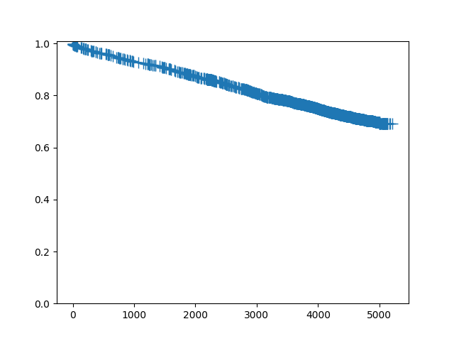
若要繪製單一生存函數,請呼叫 plot 方法
In [8]: sf.plot()
Out[8]: <Figure size 640x480 with 1 Axes>
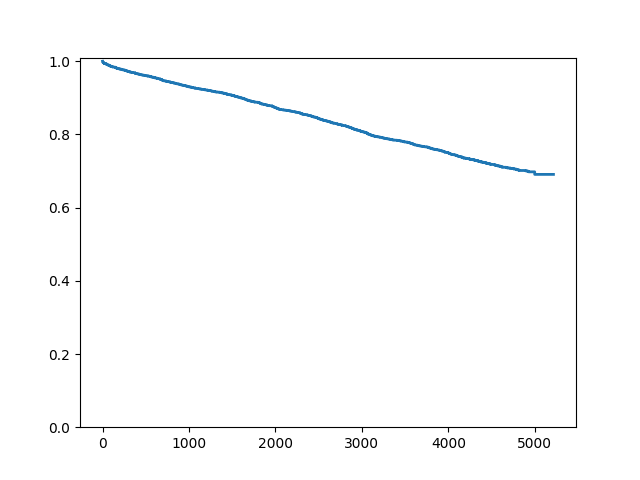
由於這是一個包含大量設限的大型資料集,我們可能不希望繪製設限符號
In [9]: fig = sf.plot()

In [10]: ax = fig.get_axes()[0]

In [11]: pt = ax.get_lines()[1]

In [12]: pt.set_visible(False)
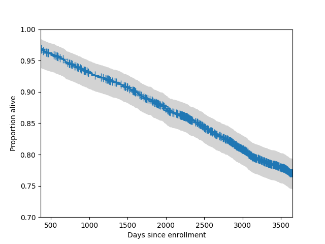
我們也可以將 95% 的同時信賴帶新增到圖中。通常,這些帶僅針對分佈的中心部分繪製。
In [13]: fig = sf.plot()

In [14]: lcb, ucb = sf.simultaneous_cb()

In [15]: ax = fig.get_axes()[0]

In [16]: ax.fill_between(sf.surv_times, lcb, ucb, color='lightgrey')
Out[16]: <matplotlib.collections.PolyCollection at 0x7f19af039cf0>

In [17]: ax.set_xlim(365, 365*10)
Out[17]: (365.0, 3650.0)

In [18]: ax.set_ylim(0.7, 1)
Out[18]: (0.7, 1.0)

In [19]: ax.set_ylabel("Proportion alive")
Out[19]: Text(0, 0.5, 'Proportion alive')

In [20]: ax.set_xlabel("Days since enrollment")
Out[20]: Text(0.5, 0, 'Days since enrollment')
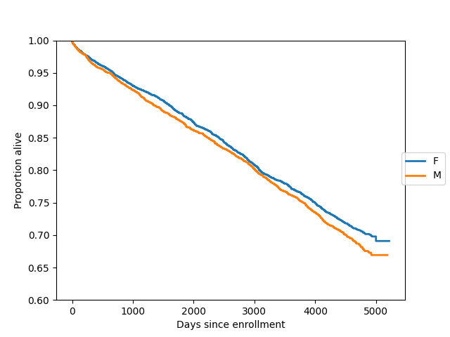
在此,我們在同一軸上繪製兩個群體(女性和男性)的生存函數
In [21]: import matplotlib.pyplot as plt

In [22]: gb = data.groupby("sex")

In [23]: ax = plt.axes()

In [24]: sexes = []

In [25]: for g in gb:
   ....:     sexes.append(g[0])
   ....:     sf = sm.SurvfuncRight(g[1]["futime"], g[1]["death"])
   ....:     sf.plot(ax)
   ....:

In [26]: li = ax.get_lines()

In [27]: li[1].set_visible(False)

In [28]: li[3].set_visible(False)

In [29]: plt.figlegend((li[0], li[2]), sexes, loc="center right")
Out[29]: <matplotlib.legend.Legend at 0x7f19aef908b0>

In [30]: plt.ylim(0.6, 1)
Out[30]: (0.6, 1.0)

In [31]: ax.set_ylabel("Proportion alive")
Out[31]: Text(0, 0.5, 'Proportion alive')

In [32]: ax.set_xlabel("Days since enrollment")
Out[32]: Text(0.5, 0, 'Days since enrollment')
我們可以透過 survdiff 正式比較兩個生存分佈,該方法實作了幾種標準的非參數程序。預設程序是對數秩檢定
In [33]: stat, pv = sm.duration.survdiff(data.futime, data.death, data.sex)
以下是 survdiff 實作的其他一些檢定程序
 # Fleming-Harrington with p=1, i.e. weight by pooled survival time
In [34]: stat, pv = sm.duration.survdiff(data.futime, data.death, data.sex, weight_type='fh', fh_p=1)

 # Gehan-Breslow, weight by number at risk
In [35]: stat, pv = sm.duration.survdiff(data.futime, data.death, data.sex, weight_type='gb')

 # Tarone-Ware, weight by the square root of the number at risk
In [36]: stat, pv = sm.duration.survdiff(data.futime, data.death, data.sex, weight_type='tw')
迴歸方法
比例風險迴歸模型(「Cox 模型」)是一種用於設限資料的迴歸技術。它們允許用共變數解釋事件發生時間的變化,這類似於線性或廣義線性迴歸模型中的做法。這些模型以「風險比」表示共變數效應,這意味著風險(瞬時事件發生率)會乘以取決於共變數值的給定因子。
In [37]: import statsmodels.api as sm

In [38]: import statsmodels.formula.api as smf

In [39]: data = sm.datasets.get_rdataset("flchain", "survival").data

In [40]: del data["chapter"]

In [41]: data = data.dropna()

In [42]: data["lam"] = data["lambda"]

In [43]: data["female"] = (data["sex"] == "F").astype(int)

In [44]: data["year"] = data["sample.yr"] - min(data["sample.yr"])

In [45]: status = data["death"].values

In [46]: mod = smf.phreg("futime ~ 0 + age + female + creatinine + np.sqrt(kappa) + np.sqrt(lam) + year + mgus", data, status=status, ties="efron")

In [47]: rslt = mod.fit()

In [48]: print(rslt.summary())
                           Results: PHReg
====================================================================
Model:                      PH Reg         Sample size:         6524
Dependent variable:         futime         Num. events:         1962
Ties:                       Efron
--------------------------------------------------------------------
                log HR log HR SE   HR      t    P>|t|  [0.025 0.975]
--------------------------------------------------------------------
age             0.1012    0.0025 1.1065 40.9289 0.0000 1.1012 1.1119
female         -0.2817    0.0474 0.7545 -5.9368 0.0000 0.6875 0.8280
creatinine      0.0134    0.0411 1.0135  0.3271 0.7436 0.9351 1.0985
np.sqrt(kappa)  0.4047    0.1147 1.4988  3.5288 0.0004 1.1971 1.8766
np.sqrt(lam)    0.7046    0.1117 2.0230  6.3056 0.0000 1.6251 2.5183
year            0.0477    0.0192 1.0489  2.4902 0.0128 1.0102 1.0890
mgus            0.3160    0.2532 1.3717  1.2479 0.2121 0.8350 2.2532
====================================================================
Confidence intervals are for the hazard ratios
請參閱 範例 以取得更詳細的範例。
Wiki 上有一些筆記本範例:PHReg 和生存分析的 Wiki 筆記本
參考文獻
Cox 比例風險迴歸模型的參考文獻
T Therneau (1996). Extending the Cox model. Technical report.
http://www.mayo.edu/research/documents/biostat-58pdf/DOC-10027288

G Rodriguez (2005). Non-parametric estimation in survival models.
http://data.princeton.edu/pop509/NonParametricSurvival.pdf

B Gillespie (2006). Checking the assumptions in the Cox proportional
hazards model.
http://www.mwsug.org/proceedings/2006/stats/MWSUG-2006-SD08.pdf
模組參考
用於處理生存分佈的類別是
|
生存函數的估計和推論。 |
比例風險迴歸模型類別是
|
Cox 比例風險迴歸模型 |
比例風險迴歸結果類別是
|
包含擬合 Cox 比例風險生存模型結果的類別。 |
主要的輔助類別是
|
表示離散分佈集合的類別。 |