線性混合效應模型
[1]:
%matplotlib inline

import numpy as np
import pandas as pd
import statsmodels.api as sm
import statsmodels.formula.api as smf
from statsmodels.tools.sm_exceptions import ConvergenceWarning
注意:此筆記本中的 R 程式碼和結果已轉換為 markdown,因此不需要 R 來建構文件。筆記本中的 R 結果是使用 R 3.5.1 和 lme4 1.1 計算得出的。
%load_ext rpy2.ipython
%R library(lme4)
array(['lme4', 'Matrix', 'tools', 'stats', 'graphics', 'grDevices',
       'utils', 'datasets', 'methods', 'base'], dtype='<U9')
比較 R lmer 與 statsmodels MixedLM
statsmodels 線性混合模型 (MixedLM) 的實作,緊密遵循 Lindstrom 和 Bates (JASA 1988) 中概述的方法。這也是 R 套件 LME4 中採用的方法。其他套件,如 Stata、SAS 等,也應與此方法一致,因為該領域的基本技術大多已成熟。
在這裡,我們展示如何使用 statsmodels 中的 MixedLM 程序擬合線性混合模型。包含來自 R (LME4) 的結果以供比較。
以下是我們的導入語句
豬隻的生長曲線
這些是來自因子實驗的縱向資料。結果變數是每隻豬的體重,我們在這裡使用的唯一預測變數是「時間」。首先,我們擬合一個將平均體重表示為時間的線性函數的模型,每隻豬有一個隨機截距。該模型使用公式指定。由於未指定隨機效應結構,因此自動使用預設隨機效應結構(每組的隨機截距)。
[2]:
data = sm.datasets.get_rdataset("dietox", "geepack").data
md = smf.mixedlm("Weight ~ Time", data, groups=data["Pig"])
mdf = md.fit(method=["lbfgs"])
print(mdf.summary())
         Mixed Linear Model Regression Results
========================================================
Model:            MixedLM Dependent Variable: Weight
No. Observations: 861     Method:             REML
No. Groups:       72      Scale:              11.3669
Min. group size:  11      Log-Likelihood:     -2404.7753
Max. group size:  12      Converged:          Yes
Mean group size:  12.0
--------------------------------------------------------
             Coef.  Std.Err.    z    P>|z| [0.025 0.975]
--------------------------------------------------------
Intercept    15.724    0.788  19.952 0.000 14.179 17.268
Time          6.943    0.033 207.939 0.000  6.877  7.008
Group Var    40.395    2.149
========================================================
這是使用 LMER 在 R 中擬合的相同模型
%%R
data(dietox, package='geepack')
%R print(summary(lmer('Weight ~ Time + (1|Pig)', data=dietox)))
Linear mixed model fit by REML ['lmerMod']
Formula: Weight ~ Time + (1 | Pig)
   Data: dietox

REML criterion at convergence: 4809.6

Scaled residuals:
    Min      1Q  Median      3Q     Max
-4.7118 -0.5696 -0.0943  0.4877  4.7732

Random effects:
 Groups   Name        Variance Std.Dev.
 Pig      (Intercept) 40.39    6.356
 Residual             11.37    3.371
Number of obs: 861, groups:  Pig, 72

Fixed effects:
            Estimate Std. Error t value
(Intercept) 15.72352    0.78805   19.95
Time         6.94251    0.03339  207.94

Correlation of Fixed Effects:
     (Intr)
Time -0.275
請注意,在 statsmodels 的結果摘要中,固定效應和隨機效應的參數估計值顯示在單個表格中。動物的隨機效應在上面的 statsmodels 輸出中標記為「截距 RE」。在 LME4 輸出中,此效應是隨機效應部分下的豬截距。
關於隨機效應變異數和共變異數參數的標準誤差是否有用,一直存在很多爭論。在 LME4 中,這些標準誤差不會顯示,因為套件的作者認為它們沒有太多參考價值。雖然有充分的理由質疑它們的實用性,但我們選擇在摘要表格中包含標準誤差,但不顯示相應的 Wald 信賴區間。
接下來,我們擬合一個模型,每隻動物有兩個隨機效應:一個隨機截距和一個隨機斜率(相對於時間)。這意味著每隻豬可能具有不同的基準體重,並且以不同的速率生長。公式指定「時間」是具有隨機係數的共變數。預設情況下,公式始終包含截距(可以使用「0 + 時間」作為公式在此處抑制)。
[3]:
md = smf.mixedlm("Weight ~ Time", data, groups=data["Pig"], re_formula="~Time")
mdf = md.fit(method=["lbfgs"])
print(mdf.summary())
           Mixed Linear Model Regression Results
===========================================================
Model:             MixedLM  Dependent Variable:  Weight
No. Observations:  861      Method:              REML
No. Groups:        72       Scale:               6.0372
Min. group size:   11       Log-Likelihood:      -2217.0475
Max. group size:   12       Converged:           Yes
Mean group size:   12.0
-----------------------------------------------------------
                 Coef.  Std.Err.   z    P>|z| [0.025 0.975]
-----------------------------------------------------------
Intercept        15.739    0.550 28.603 0.000 14.660 16.817
Time              6.939    0.080 86.925 0.000  6.783  7.095
Group Var        19.503    1.561
Group x Time Cov  0.294    0.153
Time Var          0.416    0.033
===========================================================
這是使用 R 中的 LMER 擬合的相同模型
%R print(summary(lmer("Weight ~ Time + (1 + Time | Pig)", data=dietox)))
Linear mixed model fit by REML ['lmerMod']
Formula: Weight ~ Time + (1 + Time | Pig)
   Data: dietox

REML criterion at convergence: 4434.1

Scaled residuals:
    Min      1Q  Median      3Q     Max
-6.4286 -0.5529 -0.0416  0.4841  3.5624

Random effects:
 Groups   Name        Variance Std.Dev. Corr
 Pig      (Intercept) 19.493   4.415
          Time         0.416   0.645    0.10
 Residual              6.038   2.457
Number of obs: 861, groups:  Pig, 72

Fixed effects:
            Estimate Std. Error t value
(Intercept) 15.73865    0.55012   28.61
Time         6.93901    0.07982   86.93

Correlation of Fixed Effects:
     (Intr)
Time 0.006
隨機截距和隨機斜率僅有微弱的相關性 \((0.294 / \sqrt{19.493 * 0.416} \approx 0.1)\)。因此,接下來我們擬合一個模型,其中兩個隨機效應被約束為不相關
[4]:
0.294 / (19.493 * 0.416) ** 0.5
[4]:
0.10324316832591753
[5]:
md = smf.mixedlm("Weight ~ Time", data, groups=data["Pig"], re_formula="~Time")
free = sm.regression.mixed_linear_model.MixedLMParams.from_components(
    np.ones(2), np.eye(2)
)

mdf = md.fit(free=free, method=["lbfgs"])
print(mdf.summary())
           Mixed Linear Model Regression Results
===========================================================
Model:             MixedLM  Dependent Variable:  Weight
No. Observations:  861      Method:              REML
No. Groups:        72       Scale:               6.0283
Min. group size:   11       Log-Likelihood:      -2217.3481
Max. group size:   12       Converged:           Yes
Mean group size:   12.0
-----------------------------------------------------------
                 Coef.  Std.Err.   z    P>|z| [0.025 0.975]
-----------------------------------------------------------
Intercept        15.739    0.554 28.388 0.000 14.652 16.825
Time              6.939    0.080 86.248 0.000  6.781  7.097
Group Var        19.837    1.571
Group x Time Cov  0.000    0.000
Time Var          0.423    0.033
===========================================================
當我們將相關參數固定為 0 時,對數概似下降 0.3。將 2 x 0.3 = 0.6 與卡方 1 自由度參考分佈進行比較,表明資料與該參數等於 0 的模型非常一致。
這是使用 R 中的 LMER 擬合的相同模型(請注意,此處 R 報告的是 REML 準則而不是對數概似,其中 REML 準則是對數概似的兩倍)
%R print(summary(lmer("Weight ~ Time + (1 | Pig) + (0 + Time | Pig)", data=dietox)))
Linear mixed model fit by REML ['lmerMod']
Formula: Weight ~ Time + (1 | Pig) + (0 + Time | Pig)
   Data: dietox

REML criterion at convergence: 4434.7

Scaled residuals:
    Min      1Q  Median      3Q     Max
-6.4281 -0.5527 -0.0405  0.4840  3.5661

Random effects:
 Groups   Name        Variance Std.Dev.
 Pig      (Intercept) 19.8404  4.4543
 Pig.1    Time         0.4234  0.6507
 Residual              6.0282  2.4552
Number of obs: 861, groups:  Pig, 72

Fixed effects:
            Estimate Std. Error t value
(Intercept) 15.73875    0.55444   28.39
Time         6.93899    0.08045   86.25

Correlation of Fixed Effects:
     (Intr)
Time -0.086
西特卡雲杉生長資料
這是 LMER R 函式庫中提供的範例資料集之一。結果變數是樹木的大小,這裡使用的共變數是時間值。資料按樹木分組。
[6]:
data = sm.datasets.get_rdataset("Sitka", "MASS").data
endog = data["size"]
data["Intercept"] = 1
exog = data[["Intercept", "Time"]]
這是 statsmodels LME 對具有隨機截距的基本模型的擬合。我們將 endog 和 exog 資料直接以陣列形式傳遞給 LME 初始化函式。另請注意,endog_re 在參數 4 中明確指定為隨機截距(儘管如果未指定,這也將是預設值)。
[7]:
md = sm.MixedLM(endog, exog, groups=data["tree"], exog_re=exog["Intercept"])
mdf = md.fit()
print(mdf.summary())
         Mixed Linear Model Regression Results
=======================================================
Model:             MixedLM Dependent Variable: size
No. Observations:  395     Method:             REML
No. Groups:        79      Scale:              0.0392
Min. group size:   5       Log-Likelihood:     -82.3884
Max. group size:   5       Converged:          Yes
Mean group size:   5.0
-------------------------------------------------------
              Coef. Std.Err.   z    P>|z| [0.025 0.975]
-------------------------------------------------------
Intercept     2.273    0.088 25.864 0.000  2.101  2.446
Time          0.013    0.000 47.796 0.000  0.012  0.013
Intercept Var 0.374    0.345
=======================================================
這是使用 LMER 在 R 中擬合的相同模型
%R
data(Sitka, package="MASS")
print(summary(lmer("size ~ Time + (1 | tree)", data=Sitka)))
Linear mixed model fit by REML ['lmerMod']
Formula: size ~ Time + (1 | tree)
   Data: Sitka

REML criterion at convergence: 164.8

Scaled residuals:
    Min      1Q  Median      3Q     Max
-2.9979 -0.5169  0.1576  0.5392  4.4012

Random effects:
 Groups   Name        Variance Std.Dev.
 tree     (Intercept) 0.37451  0.612
 Residual             0.03921  0.198
Number of obs: 395, groups:  tree, 79

Fixed effects:
             Estimate Std. Error t value
(Intercept) 2.2732443  0.0878955   25.86
Time        0.0126855  0.0002654   47.80

Correlation of Fixed Effects:
     (Intr)
Time -0.611
我們現在可以嘗試加入隨機斜率。這次我們從 R 開始。從下面的程式碼和輸出中,我們看到隨機斜率的變異數的 REML 估計值幾乎為零。
%R print(summary(lmer("size ~ Time + (1 + Time | tree)", data=Sitka)))
Linear mixed model fit by REML ['lmerMod']
Formula: size ~ Time + (1 + Time | tree)
   Data: Sitka

REML criterion at convergence: 153.4

Scaled residuals:
    Min      1Q  Median      3Q     Max
-2.7609 -0.5173  0.1188  0.5270  3.5466

Random effects:
 Groups   Name        Variance  Std.Dev. Corr
 tree     (Intercept) 2.217e-01 0.470842
          Time        3.288e-06 0.001813 -0.17
 Residual             3.634e-02 0.190642
Number of obs: 395, groups:  tree, 79

Fixed effects:
            Estimate Std. Error t value
(Intercept) 2.273244   0.074655   30.45
Time        0.012686   0.000327   38.80

Correlation of Fixed Effects:
     (Intr)
Time -0.615
convergence code: 0
Model failed to converge with max|grad| = 0.793203 (tol = 0.002, component 1)
Model is nearly unidentifiable: very large eigenvalue
 - Rescale variables?
如果我們在預設情況下使用 statsmodels LME 執行此操作,我們會發現變異數估計值確實非常小,這會導致有關解位於參數空間邊界的警告。迴歸斜率與 R 非常一致,但概似值遠高於 R 返回的值。
[8]:
exog_re = exog.copy()
md = sm.MixedLM(endog, exog, data["tree"], exog_re)
mdf = md.fit()
print(mdf.summary())
/opt/hostedtoolcache/Python/3.10.15/x64/lib/python3.10/site-packages/statsmodels/regression/mixed_linear_model.py:2237: ConvergenceWarning: The MLE may be on the boundary of the parameter space.
  warnings.warn(msg, ConvergenceWarning)
             Mixed Linear Model Regression Results
===============================================================
Model:               MixedLM    Dependent Variable:    size
No. Observations:    395        Method:                REML
No. Groups:          79         Scale:                 0.0264
Min. group size:     5          Log-Likelihood:        -62.4834
Max. group size:     5          Converged:             Yes
Mean group size:     5.0
---------------------------------------------------------------
                     Coef.  Std.Err.   z    P>|z| [0.025 0.975]
---------------------------------------------------------------
Intercept             2.273    0.101 22.513 0.000  2.075  2.471
Time                  0.013    0.000 33.888 0.000  0.012  0.013
Intercept Var         0.646    0.914
Intercept x Time Cov -0.001    0.003
Time Var              0.000    0.000
===============================================================
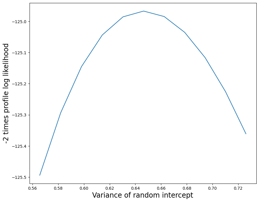
我們可以透過建構輪廓概似圖來進一步探索隨機效應結構。我們從隨機截距開始,產生一個輪廓概似圖,該圖從 MLE 下方 0.1 個單位到 MLE 上方 0.1 個單位。由於輪廓概似內部的每次最佳化都會產生警告(由於隨機斜率變異數接近於零),因此我們在此處關閉警告。
[9]:
import warnings

with warnings.catch_warnings():
    warnings.filterwarnings("ignore")
    likev = mdf.profile_re(0, "re", dist_low=0.1, dist_high=0.1)
這是輪廓概似函式的圖。我們將對數概似差乘以 2 以獲得具有 1 個自由度的通常 \(\chi^2\) 參考分佈。
[10]:
import matplotlib.pyplot as plt
[11]:
plt.figure(figsize=(10, 8))
plt.plot(likev[:, 0], 2 * likev[:, 1])
plt.xlabel("Variance of random intercept", size=17)
plt.ylabel("-2 times profile log likelihood", size=17)
[11]:
Text(0, 0.5, '-2 times profile log likelihood')
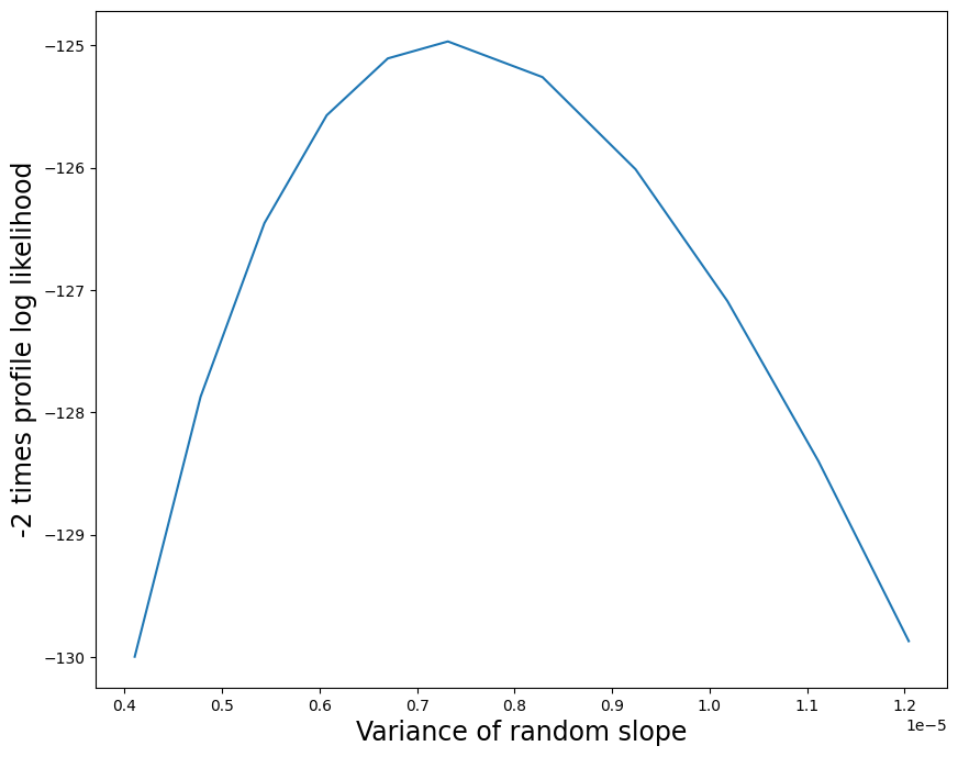
這是輪廓概似函式的圖。輪廓概似圖顯示隨機斜率變異數參數的 MLE 是一個非常小的正數,並且此估計值的不確定性很低。
[12]:
re = mdf.cov_re.iloc[1, 1]
with warnings.catch_warnings():
    # Parameter is often on the boundary
    warnings.simplefilter("ignore", ConvergenceWarning)
    likev = mdf.profile_re(1, "re", dist_low=0.5 * re, dist_high=0.8 * re)

plt.figure(figsize=(10, 8))
plt.plot(likev[:, 0], 2 * likev[:, 1])
plt.xlabel("Variance of random slope", size=17)
lbl = plt.ylabel("-2 times profile log likelihood", size=17)