加權最小平方法
[1]:
%matplotlib inline
[2]:
import matplotlib.pyplot as plt
import numpy as np
import statsmodels.api as sm
from scipy import stats
from statsmodels.iolib.table import SimpleTable, default_txt_fmt

np.random.seed(1024)
WLS 估計
人工數據:異方差 2 個群組
模型假設
模型設定錯誤:真實模型是二次的,只估計線性
獨立的雜訊/誤差項
誤差變異數的兩個群組,低變異數和高變異數群組
[3]:
nsample = 50
x = np.linspace(0, 20, nsample)
X = np.column_stack((x, (x - 5) ** 2))
X = sm.add_constant(X)
beta = [5.0, 0.5, -0.01]
sig = 0.5
w = np.ones(nsample)
w[nsample * 6 // 10 :] = 3
y_true = np.dot(X, beta)
e = np.random.normal(size=nsample)
y = y_true + sig * w * e
X = X[:, [0, 1]]
在已知異方差的真實變異數比率下進行 WLS
在這個範例中,w 是誤差的標準差。WLS 要求權重與誤差變異數的倒數成比例。
[4]:
mod_wls = sm.WLS(y, X, weights=1.0 / (w ** 2))
res_wls = mod_wls.fit()
print(res_wls.summary())
                            WLS Regression Results
==============================================================================
Dep. Variable:                      y   R-squared:                       0.927
Model:                            WLS   Adj. R-squared:                  0.926
Method:                 Least Squares   F-statistic:                     613.2
Date:                Thu, 03 Oct 2024   Prob (F-statistic):           5.44e-29
Time:                        15:46:01   Log-Likelihood:                -51.136
No. Observations:                  50   AIC:                             106.3
Df Residuals:                      48   BIC:                             110.1
Df Model:                           1
Covariance Type:            nonrobust
==============================================================================
                 coef    std err          t      P>|t|      [0.025      0.975]
------------------------------------------------------------------------------
const          5.2469      0.143     36.790      0.000       4.960       5.534
x1             0.4466      0.018     24.764      0.000       0.410       0.483
==============================================================================
Omnibus:                        0.407   Durbin-Watson:                   2.317
Prob(Omnibus):                  0.816   Jarque-Bera (JB):                0.103
Skew:                          -0.104   Prob(JB):                        0.950
Kurtosis:                       3.075   Cond. No.                         14.6
==============================================================================

Notes:
[1] Standard Errors assume that the covariance matrix of the errors is correctly specified.
OLS 與 WLS
估計一個 OLS 模型以進行比較
[5]:
res_ols = sm.OLS(y, X).fit()
print(res_ols.params)
print(res_wls.params)
[5.24256099 0.43486879]
[5.24685499 0.44658241]
比較 WLS 的標準誤差與異方差校正的 OLS 標準誤差
[6]:
se = np.vstack(
    [
        [res_wls.bse],
        [res_ols.bse],
        [res_ols.HC0_se],
        [res_ols.HC1_se],
        [res_ols.HC2_se],
        [res_ols.HC3_se],
    ]
)
se = np.round(se, 4)
colnames = ["x1", "const"]
rownames = ["WLS", "OLS", "OLS_HC0", "OLS_HC1", "OLS_HC3", "OLS_HC3"]
tabl = SimpleTable(se, colnames, rownames, txt_fmt=default_txt_fmt)
print(tabl)
=====================
          x1   const
---------------------
WLS     0.1426  0.018
OLS     0.2707 0.0233
OLS_HC0  0.194 0.0281
OLS_HC1  0.198 0.0287
OLS_HC3 0.2003  0.029
OLS_HC3  0.207   0.03
---------------------
計算 OLS 預測區間
[7]:
covb = res_ols.cov_params()
prediction_var = res_ols.mse_resid + (X * np.dot(covb, X.T).T).sum(1)
prediction_std = np.sqrt(prediction_var)
tppf = stats.t.ppf(0.975, res_ols.df_resid)
[8]:
pred_ols = res_ols.get_prediction()
iv_l_ols = pred_ols.summary_frame()["obs_ci_lower"]
iv_u_ols = pred_ols.summary_frame()["obs_ci_upper"]
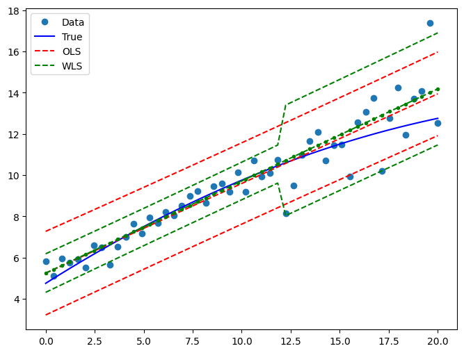
繪製圖表以比較 WLS 和 OLS 中的預測值
[9]:
pred_wls = res_wls.get_prediction()
iv_l = pred_wls.summary_frame()["obs_ci_lower"]
iv_u = pred_wls.summary_frame()["obs_ci_upper"]

fig, ax = plt.subplots(figsize=(8, 6))
ax.plot(x, y, "o", label="Data")
ax.plot(x, y_true, "b-", label="True")
# OLS
ax.plot(x, res_ols.fittedvalues, "r--")
ax.plot(x, iv_u_ols, "r--", label="OLS")
ax.plot(x, iv_l_ols, "r--")
# WLS
ax.plot(x, res_wls.fittedvalues, "g--.")
ax.plot(x, iv_u, "g--", label="WLS")
ax.plot(x, iv_l, "g--")
ax.legend(loc="best")
[9]:
<matplotlib.legend.Legend at 0x7f060e83c340>
可行加權最小平方法 (2 階段 FWLS)
像 w 一樣,w_est 與標準差成比例,因此必須平方。
[10]:
resid1 = res_ols.resid[w == 1.0]
var1 = resid1.var(ddof=int(res_ols.df_model) + 1)
resid2 = res_ols.resid[w != 1.0]
var2 = resid2.var(ddof=int(res_ols.df_model) + 1)
w_est = w.copy()
w_est[w != 1.0] = np.sqrt(var2) / np.sqrt(var1)
res_fwls = sm.WLS(y, X, 1.0 / ((w_est ** 2))).fit()
print(res_fwls.summary())
                            WLS Regression Results
==============================================================================
Dep. Variable:                      y   R-squared:                       0.931
Model:                            WLS   Adj. R-squared:                  0.929
Method:                 Least Squares   F-statistic:                     646.7
Date:                Thu, 03 Oct 2024   Prob (F-statistic):           1.66e-29
Time:                        15:46:02   Log-Likelihood:                -50.716
No. Observations:                  50   AIC:                             105.4
Df Residuals:                      48   BIC:                             109.3
Df Model:                           1
Covariance Type:            nonrobust
==============================================================================
                 coef    std err          t      P>|t|      [0.025      0.975]
------------------------------------------------------------------------------
const          5.2363      0.135     38.720      0.000       4.964       5.508
x1             0.4492      0.018     25.431      0.000       0.414       0.485
==============================================================================
Omnibus:                        0.247   Durbin-Watson:                   2.343
Prob(Omnibus):                  0.884   Jarque-Bera (JB):                0.179
Skew:                          -0.136   Prob(JB):                        0.915
Kurtosis:                       2.893   Cond. No.                         14.3
==============================================================================

Notes:
[1] Standard Errors assume that the covariance matrix of the errors is correctly specified.
最後更新:2024 年 10 月 03 日