遞迴最小平方法
遞迴最小平方法是普通最小平方法的一個擴展視窗版本。除了可以遞迴計算迴歸係數外,遞迴計算的殘差還可被用來建構統計量,以研究參數不穩定性。
RecursiveLS 類別允許計算遞迴殘差,並計算 CUSUM 和 CUSUM 平方統計量。將這些統計量與表示統計上顯著偏離參數穩定零假設的參考線一起繪製,可以輕鬆地視覺指示參數穩定性。
最後,RecursiveLS 模型允許對參數向量施加線性限制,並且可以使用公式介面構建。
[1]:
%matplotlib inline
import matplotlib.pyplot as plt
import numpy as np
import pandas as pd
import statsmodels.api as sm
from pandas_datareader.data import DataReader

np.set_printoptions(suppress=True)
範例 1:銅
首先,我們考慮銅數據集中參數的穩定性(描述如下)。
[2]:
print(sm.datasets.copper.DESCRLONG)

dta = sm.datasets.copper.load_pandas().data
dta.index = pd.date_range("1951-01-01", "1975-01-01", freq="YS")
endog = dta["WORLDCONSUMPTION"]

# To the regressors in the dataset, we add a column of ones for an intercept
exog = sm.add_constant(
    dta[["COPPERPRICE", "INCOMEINDEX", "ALUMPRICE", "INVENTORYINDEX"]]
)
This data describes the world copper market from 1951 through 1975.  In an
example, in Gill, the outcome variable (of a 2 stage estimation) is the world
consumption of copper for the 25 years.  The explanatory variables are the
world consumption of copper in 1000 metric tons, the constant dollar adjusted
price of copper, the price of a substitute, aluminum, an index of real per
capita income base 1970, an annual measure of manufacturer inventory change,
and a time trend.
首先,構建並擬合模型,並列印摘要。儘管 RLS 模型會遞迴計算迴歸參數,因此估計值數量與資料點數量一樣多,但摘要表僅呈現根據整個樣本估計的迴歸參數;除了遞迴初始化的微小影響外,這些估計值與 OLS 估計值等效。
[3]:
mod = sm.RecursiveLS(endog, exog)
res = mod.fit()

print(res.summary())
                           Statespace Model Results
==============================================================================
Dep. Variable:       WORLDCONSUMPTION   No. Observations:                   25
Model:                    RecursiveLS   Log Likelihood                -154.720
Date:                Thu, 03 Oct 2024   R-squared:                       0.965
Time:                        15:46:06   AIC                            319.441
Sample:                    01-01-1951   BIC                            325.535
                         - 01-01-1975   HQIC                           321.131
Covariance Type:            nonrobust   Scale                       117717.127
==================================================================================
                     coef    std err          z      P>|z|      [0.025      0.975]
----------------------------------------------------------------------------------
const          -6562.3719   2378.939     -2.759      0.006   -1.12e+04   -1899.737
COPPERPRICE      -13.8132     15.041     -0.918      0.358     -43.292      15.666
INCOMEINDEX      1.21e+04    763.401     15.853      0.000    1.06e+04    1.36e+04
ALUMPRICE         70.4146     32.678      2.155      0.031       6.367     134.462
INVENTORYINDEX   311.7330   2130.084      0.146      0.884   -3863.155    4486.621
===================================================================================
Ljung-Box (L1) (Q):                   2.17   Jarque-Bera (JB):                 1.70
Prob(Q):                              0.14   Prob(JB):                         0.43
Heteroskedasticity (H):               3.38   Skew:                            -0.67
Prob(H) (two-sided):                  0.13   Kurtosis:                         2.53
===================================================================================

Warnings:
[1] Parameters and covariance matrix estimates are RLS estimates conditional on the entire sample.
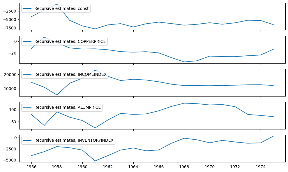
遞迴係數可在 recursive_coefficients 屬性中取得。或者,可以使用 plot_recursive_coefficient 方法生成繪圖。
[4]:
print(res.recursive_coefficients.filtered[0])
res.plot_recursive_coefficient(range(mod.k_exog), alpha=None, figsize=(10, 6))
[     2.88890087      4.94795049   1558.41803044   1958.43326658
 -51474.9578655   -4168.94974192  -2252.61351128   -446.55908507
  -5288.39794736  -6942.31935786  -7846.0890355   -6643.15121393
  -6274.11015558  -7272.01696292  -6319.02648554  -5822.23929148
  -6256.30902754  -6737.4044603   -6477.42841448  -5995.90746904
  -6450.80677813  -6022.92166487  -5258.35152753  -5320.89136363
  -6562.37193573]
[4]:

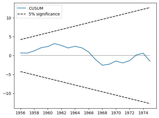
CUSUM 統計量可在 cusum 屬性中取得,但通常使用 plot_cusum 方法視覺檢查參數穩定性更方便。在下面的繪圖中,CUSUM 統計量沒有超出 5% 的顯著性範圍,因此我們無法拒絕參數在 5% 水平上穩定的零假設。
[5]:
print(res.cusum)
fig = res.plot_cusum()
[ 0.69971508  0.65841244  1.24629674  2.05476032  2.39888918  3.1786198
  2.67244672  2.01783215  2.46131747  2.05268638  0.95054336 -1.04505546
 -2.55465286 -2.29908152 -1.45289492 -1.95353993 -1.3504662   0.15789829
  0.6328653  -1.48184586]
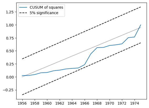
另一個相關的統計量是 CUSUM 平方。它可在 cusum_squares 屬性中取得,但同樣地,使用 plot_cusum_squares 方法視覺檢查更方便。在下面的繪圖中,CUSUM 平方統計量沒有超出 5% 的顯著性範圍,因此我們無法拒絕參數在 5% 水平上穩定的零假設。
[6]:
res.plot_cusum_squares()
[6]:

範例 2:貨幣數量理論
貨幣數量理論認為「貨幣數量變化率的既定變化會導致...價格通貨膨脹率的相等變化」(Lucas, 1980)。 繼 Lucas 之後,我們檢視貨幣成長和 CPI 通貨膨脹雙邊指數加權移動平均值之間的關係。 儘管 Lucas 發現這些變數之間的關係是穩定的,但最近這種關係似乎變得不穩定;請參閱例如 Sargent 和 Surico (2010)。
[7]:
start = "1959-12-01"
end = "2015-01-01"
m2 = DataReader("M2SL", "fred", start=start, end=end)
cpi = DataReader("CPIAUCSL", "fred", start=start, end=end)
[8]:
def ewma(series, beta, n_window):
    nobs = len(series)
    scalar = (1 - beta) / (1 + beta)
    ma = []
    k = np.arange(n_window, 0, -1)
    weights = np.r_[beta ** k, 1, beta ** k[::-1]]
    for t in range(n_window, nobs - n_window):
        window = series.iloc[t - n_window : t + n_window + 1].values
        ma.append(scalar * np.sum(weights * window))
    return pd.Series(ma, name=series.name, index=series.iloc[n_window:-n_window].index)


m2_ewma = ewma(np.log(m2["M2SL"].resample("QS").mean()).diff().iloc[1:], 0.95, 10 * 4)
cpi_ewma = ewma(
    np.log(cpi["CPIAUCSL"].resample("QS").mean()).diff().iloc[1:], 0.95, 10 * 4
)
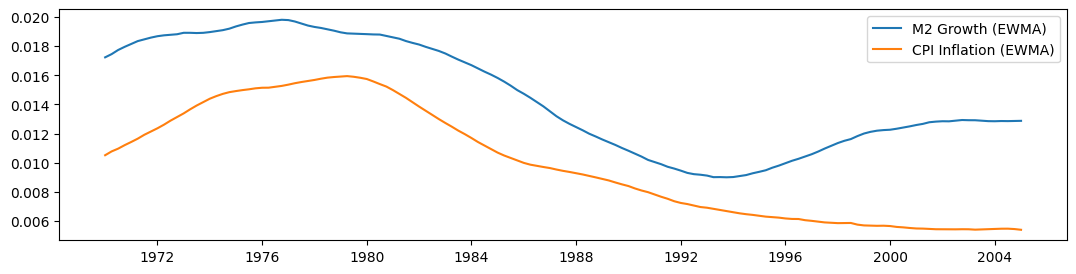
在使用 Lucas 的 \(\beta = 0.95\) 濾波器(兩側視窗為 10 年)構建移動平均值後,我們在下方繪製每個數列。 儘管它們在樣本的一部分之前似乎一起移動,但在 1990 年之後,它們似乎出現分歧。
[9]:
fig, ax = plt.subplots(figsize=(13, 3))

ax.plot(m2_ewma, label="M2 Growth (EWMA)")
ax.plot(cpi_ewma, label="CPI Inflation (EWMA)")
ax.legend()
[9]:
<matplotlib.legend.Legend at 0x7f6e8ca133a0>
[10]:
endog = cpi_ewma
exog = sm.add_constant(m2_ewma)
exog.columns = ["const", "M2"]

mod = sm.RecursiveLS(endog, exog)
res = mod.fit()

print(res.summary())
                           Statespace Model Results
==============================================================================
Dep. Variable:               CPIAUCSL   No. Observations:                  141
Model:                    RecursiveLS   Log Likelihood                 692.878
Date:                Thu, 03 Oct 2024   R-squared:                       0.813
Time:                        15:46:11   AIC                          -1381.755
Sample:                    01-01-1970   BIC                          -1375.858
                         - 01-01-2005   HQIC                         -1379.358
Covariance Type:            nonrobust   Scale                            0.000
==============================================================================
                 coef    std err          z      P>|z|      [0.025      0.975]
------------------------------------------------------------------------------
const         -0.0034      0.001     -6.013      0.000      -0.004      -0.002
M2             0.9128      0.037     24.601      0.000       0.840       0.986
===================================================================================
Ljung-Box (L1) (Q):                 138.23   Jarque-Bera (JB):                18.20
Prob(Q):                              0.00   Prob(JB):                         0.00
Heteroskedasticity (H):               5.30   Skew:                            -0.81
Prob(H) (two-sided):                  0.00   Kurtosis:                         2.27
===================================================================================

Warnings:
[1] Parameters and covariance matrix estimates are RLS estimates conditional on the entire sample.
[11]:
res.plot_recursive_coefficient(1, alpha=None)
[11]:
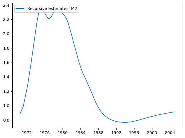

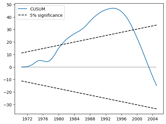
CUSUM 繪圖現在顯示 5% 水平的顯著偏差,表明拒絕參數穩定性的零假設。
[12]:
res.plot_cusum()
[12]:

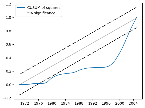
同樣地,CUSUM 平方顯示 5% 水平的顯著偏差,也表明拒絕參數穩定性的零假設。
[13]:
res.plot_cusum_squares()
[13]:

範例 3:線性限制和公式
線性限制
使用構建模型中的 constraints 參數,不難實現線性限制。
[14]:
endog = dta["WORLDCONSUMPTION"]
exog = sm.add_constant(
    dta[["COPPERPRICE", "INCOMEINDEX", "ALUMPRICE", "INVENTORYINDEX"]]
)

mod = sm.RecursiveLS(endog, exog, constraints="COPPERPRICE = ALUMPRICE")
res = mod.fit()
print(res.summary())
                           Statespace Model Results
==============================================================================
Dep. Variable:       WORLDCONSUMPTION   No. Observations:                   25
Model:                    RecursiveLS   Log Likelihood                -134.231
Date:                Thu, 03 Oct 2024   R-squared:                       0.989
Time:                        15:46:14   AIC                            276.462
Sample:                    01-01-1951   BIC                            281.338
                         - 01-01-1975   HQIC                           277.814
Covariance Type:            nonrobust   Scale                       137155.014
==================================================================================
                     coef    std err          z      P>|z|      [0.025      0.975]
----------------------------------------------------------------------------------
const          -4839.4836   2412.410     -2.006      0.045   -9567.721    -111.246
COPPERPRICE        5.9797     12.704      0.471      0.638     -18.921      30.880
INCOMEINDEX     1.115e+04    666.308     16.738      0.000    9847.000    1.25e+04
ALUMPRICE          5.9797     12.704      0.471      0.638     -18.921      30.880
INVENTORYINDEX   241.3452   2298.951      0.105      0.916   -4264.515    4747.206
===================================================================================
Ljung-Box (L1) (Q):                   6.27   Jarque-Bera (JB):                 1.78
Prob(Q):                              0.01   Prob(JB):                         0.41
Heteroskedasticity (H):               1.75   Skew:                            -0.63
Prob(H) (two-sided):                  0.48   Kurtosis:                         2.32
===================================================================================

Warnings:
[1] Parameters and covariance matrix estimates are RLS estimates conditional on the entire sample.
公式
可以使用類別方法 from_formula 擬合相同的模型。
[15]:
mod = sm.RecursiveLS.from_formula(
    "WORLDCONSUMPTION ~ COPPERPRICE + INCOMEINDEX + ALUMPRICE + INVENTORYINDEX",
    dta,
    constraints="COPPERPRICE = ALUMPRICE",
)
res = mod.fit()
print(res.summary())
                           Statespace Model Results
==============================================================================
Dep. Variable:       WORLDCONSUMPTION   No. Observations:                   25
Model:                    RecursiveLS   Log Likelihood                -134.231
Date:                Thu, 03 Oct 2024   R-squared:                       0.989
Time:                        15:46:14   AIC                            276.462
Sample:                    01-01-1951   BIC                            281.338
                         - 01-01-1975   HQIC                           277.814
Covariance Type:            nonrobust   Scale                       137155.014
==================================================================================
                     coef    std err          z      P>|z|      [0.025      0.975]
----------------------------------------------------------------------------------
Intercept      -4839.4836   2412.410     -2.006      0.045   -9567.721    -111.246
COPPERPRICE        5.9797     12.704      0.471      0.638     -18.921      30.880
INCOMEINDEX     1.115e+04    666.308     16.738      0.000    9847.000    1.25e+04
ALUMPRICE          5.9797     12.704      0.471      0.638     -18.921      30.880
INVENTORYINDEX   241.3452   2298.951      0.105      0.916   -4264.515    4747.206
===================================================================================
Ljung-Box (L1) (Q):                   6.27   Jarque-Bera (JB):                 1.78
Prob(Q):                              0.01   Prob(JB):                         0.41
Heteroskedasticity (H):               1.75   Skew:                            -0.63
Prob(H) (two-sided):                  0.48   Kurtosis:                         2.32
===================================================================================

Warnings:
[1] Parameters and covariance matrix estimates are RLS estimates conditional on the entire sample.
/opt/hostedtoolcache/Python/3.10.15/x64/lib/python3.10/site-packages/statsmodels/tsa/base/tsa_model.py:473: ValueWarning: No frequency information was provided, so inferred frequency YS-JAN will be used.
  self._init_dates(dates, freq)