時間序列模型中的確定性項
[1]:
import matplotlib.pyplot as plt
import numpy as np
import pandas as pd

plt.rc("figure", figsize=(16, 9))
plt.rc("font", size=16)
基本使用
基本配置可以直接透過 DeterministicProcess 建構。這些可以包含一個常數、任意階的時間趨勢,以及一個季節性或傅立葉分量。
此過程需要一個索引,即完整樣本(或樣本內)的索引。
首先,我們初始化一個確定性過程,其中包含常數、線性時間趨勢和 5 個週期的季節項。in_sample 方法會傳回與索引相符的完整值集。
[2]:
from statsmodels.tsa.deterministic import DeterministicProcess

index = pd.RangeIndex(0, 100)
det_proc = DeterministicProcess(index, constant=True, order=1, seasonal=True, period=5)
det_proc.in_sample()
[2]:
| 常數 | 趨勢 | s(2,5) | s(3,5) | s(4,5) | s(5,5) | |
|---|---|---|---|---|---|---|
| 0 | 1.0 | 1.0 | 0.0 | 0.0 | 0.0 | 0.0 |
| 1 | 1.0 | 2.0 | 1.0 | 0.0 | 0.0 | 0.0 |
| 2 | 1.0 | 3.0 | 0.0 | 1.0 | 0.0 | 0.0 |
| 3 | 1.0 | 4.0 | 0.0 | 0.0 | 1.0 | 0.0 |
| 4 | 1.0 | 5.0 | 0.0 | 0.0 | 0.0 | 1.0 |
| ... | ... | ... | ... | ... | ... | ... |
| 95 | 1.0 | 96.0 | 0.0 | 0.0 | 0.0 | 0.0 |
| 96 | 1.0 | 97.0 | 1.0 | 0.0 | 0.0 | 0.0 |
| 97 | 1.0 | 98.0 | 0.0 | 1.0 | 0.0 | 0.0 |
| 98 | 1.0 | 99.0 | 0.0 | 0.0 | 1.0 | 0.0 |
| 99 | 1.0 | 100.0 | 0.0 | 0.0 | 0.0 | 1.0 |
100 列 × 6 欄
out_of_sample 會傳回樣本內結束之後的下 steps 個值。
[3]:
det_proc.out_of_sample(15)
[3]:
| 常數 | 趨勢 | s(2,5) | s(3,5) | s(4,5) | s(5,5) | |
|---|---|---|---|---|---|---|
| 100 | 1.0 | 101.0 | 0.0 | 0.0 | 0.0 | 0.0 |
| 101 | 1.0 | 102.0 | 1.0 | 0.0 | 0.0 | 0.0 |
| 102 | 1.0 | 103.0 | 0.0 | 1.0 | 0.0 | 0.0 |
| 103 | 1.0 | 104.0 | 0.0 | 0.0 | 1.0 | 0.0 |
| 104 | 1.0 | 105.0 | 0.0 | 0.0 | 0.0 | 1.0 |
| 105 | 1.0 | 106.0 | 0.0 | 0.0 | 0.0 | 0.0 |
| 106 | 1.0 | 107.0 | 1.0 | 0.0 | 0.0 | 0.0 |
| 107 | 1.0 | 108.0 | 0.0 | 1.0 | 0.0 | 0.0 |
| 108 | 1.0 | 109.0 | 0.0 | 0.0 | 1.0 | 0.0 |
| 109 | 1.0 | 110.0 | 0.0 | 0.0 | 0.0 | 1.0 |
| 110 | 1.0 | 111.0 | 0.0 | 0.0 | 0.0 | 0.0 |
| 111 | 1.0 | 112.0 | 1.0 | 0.0 | 0.0 | 0.0 |
| 112 | 1.0 | 113.0 | 0.0 | 1.0 | 0.0 | 0.0 |
| 113 | 1.0 | 114.0 | 0.0 | 0.0 | 1.0 | 0.0 |
| 114 | 1.0 | 115.0 | 0.0 | 0.0 | 0.0 | 1.0 |
range(start, stop) 也可用於產生任何範圍(包括樣本內和樣本外)的確定性項。
注意事項
當索引是 pandas 的
DatetimeIndex或PeriodIndex時,start和stop可以是日期式 (字串,例如「2020-06-01」,或時間戳記) 或整數。stop始終包含在範圍中。雖然這不是非常 Pythonic,但由於 statsmodels 和 Pandas 在處理日期式切片時都會包含stop,因此這是必需的。
[4]:
det_proc.range(190, 210)
[4]:
| 常數 | 趨勢 | s(2,5) | s(3,5) | s(4,5) | s(5,5) | |
|---|---|---|---|---|---|---|
| 190 | 1.0 | 191.0 | 0.0 | 0.0 | 0.0 | 0.0 |
| 191 | 1.0 | 192.0 | 1.0 | 0.0 | 0.0 | 0.0 |
| 192 | 1.0 | 193.0 | 0.0 | 1.0 | 0.0 | 0.0 |
| 193 | 1.0 | 194.0 | 0.0 | 0.0 | 1.0 | 0.0 |
| 194 | 1.0 | 195.0 | 0.0 | 0.0 | 0.0 | 1.0 |
| 195 | 1.0 | 196.0 | 0.0 | 0.0 | 0.0 | 0.0 |
| 196 | 1.0 | 197.0 | 1.0 | 0.0 | 0.0 | 0.0 |
| 197 | 1.0 | 198.0 | 0.0 | 1.0 | 0.0 | 0.0 |
| 198 | 1.0 | 199.0 | 0.0 | 0.0 | 1.0 | 0.0 |
| 199 | 1.0 | 200.0 | 0.0 | 0.0 | 0.0 | 1.0 |
| 200 | 1.0 | 201.0 | 0.0 | 0.0 | 0.0 | 0.0 |
| 201 | 1.0 | 202.0 | 1.0 | 0.0 | 0.0 | 0.0 |
| 202 | 1.0 | 203.0 | 0.0 | 1.0 | 0.0 | 0.0 |
| 203 | 1.0 | 204.0 | 0.0 | 0.0 | 1.0 | 0.0 |
| 204 | 1.0 | 205.0 | 0.0 | 0.0 | 0.0 | 1.0 |
| 205 | 1.0 | 206.0 | 0.0 | 0.0 | 0.0 | 0.0 |
| 206 | 1.0 | 207.0 | 1.0 | 0.0 | 0.0 | 0.0 |
| 207 | 1.0 | 208.0 | 0.0 | 1.0 | 0.0 | 0.0 |
| 208 | 1.0 | 209.0 | 0.0 | 0.0 | 1.0 | 0.0 |
| 209 | 1.0 | 210.0 | 0.0 | 0.0 | 0.0 | 1.0 |
| 210 | 1.0 | 211.0 | 0.0 | 0.0 | 0.0 | 0.0 |
使用日期式索引
接下來,我們顯示使用 PeriodIndex 的相同步驟。
[5]:
index = pd.period_range("2020-03-01", freq="M", periods=60)
det_proc = DeterministicProcess(index, constant=True, fourier=2)
det_proc.in_sample().head(12)
[5]:
| 常數 | sin(1,12) | cos(1,12) | sin(2,12) | cos(2,12) | |
|---|---|---|---|---|---|
| 2020-03 | 1.0 | 0.000000e+00 | 1.000000e+00 | 0.000000e+00 | 1.0 |
| 2020-04 | 1.0 | 5.000000e-01 | 8.660254e-01 | 8.660254e-01 | 0.5 |
| 2020-05 | 1.0 | 8.660254e-01 | 5.000000e-01 | 8.660254e-01 | -0.5 |
| 2020-06 | 1.0 | 1.000000e+00 | 6.123234e-17 | 1.224647e-16 | -1.0 |
| 2020-07 | 1.0 | 8.660254e-01 | -5.000000e-01 | -8.660254e-01 | -0.5 |
| 2020-08 | 1.0 | 5.000000e-01 | -8.660254e-01 | -8.660254e-01 | 0.5 |
| 2020-09 | 1.0 | 1.224647e-16 | -1.000000e+00 | -2.449294e-16 | 1.0 |
| 2020-10 | 1.0 | -5.000000e-01 | -8.660254e-01 | 8.660254e-01 | 0.5 |
| 2020-11 | 1.0 | -8.660254e-01 | -5.000000e-01 | 8.660254e-01 | -0.5 |
| 2020-12 | 1.0 | -1.000000e+00 | -1.836970e-16 | 3.673940e-16 | -1.0 |
| 2021-01 | 1.0 | -8.660254e-01 | 5.000000e-01 | -8.660254e-01 | -0.5 |
| 2021-02 | 1.0 | -5.000000e-01 | 8.660254e-01 | -8.660254e-01 | 0.5 |
[6]:
det_proc.out_of_sample(12)
[6]:
| 常數 | sin(1,12) | cos(1,12) | sin(2,12) | cos(2,12) | |
|---|---|---|---|---|---|
| 2025-03 | 1.0 | -1.224647e-15 | 1.000000e+00 | -2.449294e-15 | 1.0 |
| 2025-04 | 1.0 | 5.000000e-01 | 8.660254e-01 | 8.660254e-01 | 0.5 |
| 2025-05 | 1.0 | 8.660254e-01 | 5.000000e-01 | 8.660254e-01 | -0.5 |
| 2025-06 | 1.0 | 1.000000e+00 | -4.904777e-16 | -9.809554e-16 | -1.0 |
| 2025-07 | 1.0 | 8.660254e-01 | -5.000000e-01 | -8.660254e-01 | -0.5 |
| 2025-08 | 1.0 | 5.000000e-01 | -8.660254e-01 | -8.660254e-01 | 0.5 |
| 2025-09 | 1.0 | 4.899825e-15 | -1.000000e+00 | -9.799650e-15 | 1.0 |
| 2025-10 | 1.0 | -5.000000e-01 | -8.660254e-01 | 8.660254e-01 | 0.5 |
| 2025-11 | 1.0 | -8.660254e-01 | -5.000000e-01 | 8.660254e-01 | -0.5 |
| 2025-12 | 1.0 | -1.000000e+00 | -3.184701e-15 | 6.369401e-15 | -1.0 |
| 2026-01 | 1.0 | -8.660254e-01 | 5.000000e-01 | -8.660254e-01 | -0.5 |
| 2026-02 | 1.0 | -5.000000e-01 | 8.660254e-01 | -8.660254e-01 | 0.5 |
range 接受日期式引數,這些引數通常以字串形式提供。
[7]:
det_proc.range("2025-01", "2026-01")
[7]:
| 常數 | sin(1,12) | cos(1,12) | sin(2,12) | cos(2,12) | |
|---|---|---|---|---|---|
| 2025-01 | 1.0 | -8.660254e-01 | 5.000000e-01 | -8.660254e-01 | -0.5 |
| 2025-02 | 1.0 | -5.000000e-01 | 8.660254e-01 | -8.660254e-01 | 0.5 |
| 2025-03 | 1.0 | -1.224647e-15 | 1.000000e+00 | -2.449294e-15 | 1.0 |
| 2025-04 | 1.0 | 5.000000e-01 | 8.660254e-01 | 8.660254e-01 | 0.5 |
| 2025-05 | 1.0 | 8.660254e-01 | 5.000000e-01 | 8.660254e-01 | -0.5 |
| 2025-06 | 1.0 | 1.000000e+00 | -4.904777e-16 | -9.809554e-16 | -1.0 |
| 2025-07 | 1.0 | 8.660254e-01 | -5.000000e-01 | -8.660254e-01 | -0.5 |
| 2025-08 | 1.0 | 5.000000e-01 | -8.660254e-01 | -8.660254e-01 | 0.5 |
| 2025-09 | 1.0 | 4.899825e-15 | -1.000000e+00 | -9.799650e-15 | 1.0 |
| 2025-10 | 1.0 | -5.000000e-01 | -8.660254e-01 | 8.660254e-01 | 0.5 |
| 2025-11 | 1.0 | -8.660254e-01 | -5.000000e-01 | 8.660254e-01 | -0.5 |
| 2025-12 | 1.0 | -1.000000e+00 | -3.184701e-15 | 6.369401e-15 | -1.0 |
| 2026-01 | 1.0 | -8.660254e-01 | 5.000000e-01 | -8.660254e-01 | -0.5 |
這相當於使用整數值 58 和 70。
[8]:
det_proc.range(58, 70)
[8]:
| 常數 | sin(1,12) | cos(1,12) | sin(2,12) | cos(2,12) | |
|---|---|---|---|---|---|
| 2025-01 | 1.0 | -8.660254e-01 | 5.000000e-01 | -8.660254e-01 | -0.5 |
| 2025-02 | 1.0 | -5.000000e-01 | 8.660254e-01 | -8.660254e-01 | 0.5 |
| 2025-03 | 1.0 | -1.224647e-15 | 1.000000e+00 | -2.449294e-15 | 1.0 |
| 2025-04 | 1.0 | 5.000000e-01 | 8.660254e-01 | 8.660254e-01 | 0.5 |
| 2025-05 | 1.0 | 8.660254e-01 | 5.000000e-01 | 8.660254e-01 | -0.5 |
| 2025-06 | 1.0 | 1.000000e+00 | -4.904777e-16 | -9.809554e-16 | -1.0 |
| 2025-07 | 1.0 | 8.660254e-01 | -5.000000e-01 | -8.660254e-01 | -0.5 |
| 2025-08 | 1.0 | 5.000000e-01 | -8.660254e-01 | -8.660254e-01 | 0.5 |
| 2025-09 | 1.0 | 4.899825e-15 | -1.000000e+00 | -9.799650e-15 | 1.0 |
| 2025-10 | 1.0 | -5.000000e-01 | -8.660254e-01 | 8.660254e-01 | 0.5 |
| 2025-11 | 1.0 | -8.660254e-01 | -5.000000e-01 | 8.660254e-01 | -0.5 |
| 2025-12 | 1.0 | -1.000000e+00 | -3.184701e-15 | 6.369401e-15 | -1.0 |
| 2026-01 | 1.0 | -8.660254e-01 | 5.000000e-01 | -8.660254e-01 | -0.5 |
進階建構
無法直接透過建構函式支援的特徵的確定性過程可以使用 additional_terms 來建立,該引數接受 DetermisticTerm 的清單。在這裡,我們建立一個具有兩個季節性分量的確定性過程:具有 5 天週期的星期幾,以及通過週期為 365.25 天的傅立葉分量捕獲的年度。
[9]:
from statsmodels.tsa.deterministic import Fourier, Seasonality, TimeTrend

index = pd.period_range("2020-03-01", freq="D", periods=2 * 365)
tt = TimeTrend(constant=True)
four = Fourier(period=365.25, order=2)
seas = Seasonality(period=7)
det_proc = DeterministicProcess(index, additional_terms=[tt, seas, four])
det_proc.in_sample().head(28)
[9]:
| 常數 | s(2,7) | s(3,7) | s(4,7) | s(5,7) | s(6,7) | s(7,7) | sin(1,365.25) | cos(1,365.25) | sin(2,365.25) | cos(2,365.25) | |
|---|---|---|---|---|---|---|---|---|---|---|---|
| 2020-03-01 | 1.0 | 0.0 | 0.0 | 0.0 | 0.0 | 0.0 | 0.0 | 0.000000 | 1.000000 | 0.000000 | 1.000000 |
| 2020-03-02 | 1.0 | 1.0 | 0.0 | 0.0 | 0.0 | 0.0 | 0.0 | 0.017202 | 0.999852 | 0.034398 | 0.999408 |
| 2020-03-03 | 1.0 | 0.0 | 1.0 | 0.0 | 0.0 | 0.0 | 0.0 | 0.034398 | 0.999408 | 0.068755 | 0.997634 |
| 2020-03-04 | 1.0 | 0.0 | 0.0 | 1.0 | 0.0 | 0.0 | 0.0 | 0.051584 | 0.998669 | 0.103031 | 0.994678 |
| 2020-03-05 | 1.0 | 0.0 | 0.0 | 0.0 | 1.0 | 0.0 | 0.0 | 0.068755 | 0.997634 | 0.137185 | 0.990545 |
| 2020-03-06 | 1.0 | 0.0 | 0.0 | 0.0 | 0.0 | 1.0 | 0.0 | 0.085906 | 0.996303 | 0.171177 | 0.985240 |
| 2020-03-07 | 1.0 | 0.0 | 0.0 | 0.0 | 0.0 | 0.0 | 1.0 | 0.103031 | 0.994678 | 0.204966 | 0.978769 |
| 2020-03-08 | 1.0 | 0.0 | 0.0 | 0.0 | 0.0 | 0.0 | 0.0 | 0.120126 | 0.992759 | 0.238513 | 0.971139 |
| 2020-03-09 | 1.0 | 1.0 | 0.0 | 0.0 | 0.0 | 0.0 | 0.0 | 0.137185 | 0.990545 | 0.271777 | 0.962360 |
| 2020-03-10 | 1.0 | 0.0 | 1.0 | 0.0 | 0.0 | 0.0 | 0.0 | 0.154204 | 0.988039 | 0.304719 | 0.952442 |
| 2020-03-11 | 1.0 | 0.0 | 0.0 | 1.0 | 0.0 | 0.0 | 0.0 | 0.171177 | 0.985240 | 0.337301 | 0.941397 |
| 2020-03-12 | 1.0 | 0.0 | 0.0 | 0.0 | 1.0 | 0.0 | 0.0 | 0.188099 | 0.982150 | 0.369484 | 0.929237 |
| 2020-03-13 | 1.0 | 0.0 | 0.0 | 0.0 | 0.0 | 1.0 | 0.0 | 0.204966 | 0.978769 | 0.401229 | 0.915978 |
| 2020-03-14 | 1.0 | 0.0 | 0.0 | 0.0 | 0.0 | 0.0 | 1.0 | 0.221772 | 0.975099 | 0.432499 | 0.901634 |
| 2020-03-15 | 1.0 | 0.0 | 0.0 | 0.0 | 0.0 | 0.0 | 0.0 | 0.238513 | 0.971139 | 0.463258 | 0.886224 |
| 2020-03-16 | 1.0 | 1.0 | 0.0 | 0.0 | 0.0 | 0.0 | 0.0 | 0.255182 | 0.966893 | 0.493468 | 0.869764 |
| 2020-03-17 | 1.0 | 0.0 | 1.0 | 0.0 | 0.0 | 0.0 | 0.0 | 0.271777 | 0.962360 | 0.523094 | 0.852275 |
| 2020-03-18 | 1.0 | 0.0 | 0.0 | 1.0 | 0.0 | 0.0 | 0.0 | 0.288291 | 0.957543 | 0.552101 | 0.833777 |
| 2020-03-19 | 1.0 | 0.0 | 0.0 | 0.0 | 1.0 | 0.0 | 0.0 | 0.304719 | 0.952442 | 0.580455 | 0.814292 |
| 2020-03-20 | 1.0 | 0.0 | 0.0 | 0.0 | 0.0 | 1.0 | 0.0 | 0.321058 | 0.947060 | 0.608121 | 0.793844 |
| 2020-03-21 | 1.0 | 0.0 | 0.0 | 0.0 | 0.0 | 0.0 | 1.0 | 0.337301 | 0.941397 | 0.635068 | 0.772456 |
| 2020-03-22 | 1.0 | 0.0 | 0.0 | 0.0 | 0.0 | 0.0 | 0.0 | 0.353445 | 0.935455 | 0.661263 | 0.750154 |
| 2020-03-23 | 1.0 | 1.0 | 0.0 | 0.0 | 0.0 | 0.0 | 0.0 | 0.369484 | 0.929237 | 0.686676 | 0.726964 |
| 2020-03-24 | 1.0 | 0.0 | 1.0 | 0.0 | 0.0 | 0.0 | 0.0 | 0.385413 | 0.922744 | 0.711276 | 0.702913 |
| 2020-03-25 | 1.0 | 0.0 | 0.0 | 1.0 | 0.0 | 0.0 | 0.0 | 0.401229 | 0.915978 | 0.735034 | 0.678031 |
| 2020-03-26 | 1.0 | 0.0 | 0.0 | 0.0 | 1.0 | 0.0 | 0.0 | 0.416926 | 0.908940 | 0.757922 | 0.652346 |
| 2020-03-27 | 1.0 | 0.0 | 0.0 | 0.0 | 0.0 | 1.0 | 0.0 | 0.432499 | 0.901634 | 0.779913 | 0.625889 |
| 2020-03-28 | 1.0 | 0.0 | 0.0 | 0.0 | 0.0 | 0.0 | 1.0 | 0.447945 | 0.894061 | 0.800980 | 0.598691 |
自訂確定性項
DetermisticTerm 抽象基礎類別旨在被子類化,以協助使用者編寫自訂確定性項。接下來,我們展示兩個範例。第一個是一個斷裂的時間趨勢,允許在固定的週期數之後中斷。第二個是一個「技巧」確定性項,它允許外生數據(實際上不是確定性過程)被視為確定性的。這讓使用簡化了收集預測所需的項。
這些旨在示範自訂項的建構。它們在輸入驗證方面絕對可以改進。
[10]:
from statsmodels.tsa.deterministic import DeterministicTerm


class BrokenTimeTrend(DeterministicTerm):
    def __init__(self, break_period: int):
        self._break_period = break_period

    def __str__(self):
        return "Broken Time Trend"

    def _eq_attr(self):
        return (self._break_period,)

    def in_sample(self, index: pd.Index):
        nobs = index.shape[0]
        terms = np.zeros((nobs, 2))
        terms[self._break_period :, 0] = 1
        terms[self._break_period :, 1] = np.arange(self._break_period + 1, nobs + 1)
        return pd.DataFrame(terms, columns=["const_break", "trend_break"], index=index)

    def out_of_sample(
        self, steps: int, index: pd.Index, forecast_index: pd.Index = None
    ):
        # Always call extend index first
        fcast_index = self._extend_index(index, steps, forecast_index)
        nobs = index.shape[0]
        terms = np.zeros((steps, 2))
        # Assume break period is in-sample
        terms[:, 0] = 1
        terms[:, 1] = np.arange(nobs + 1, nobs + steps + 1)
        return pd.DataFrame(
            terms, columns=["const_break", "trend_break"], index=fcast_index
        )
[11]:
btt = BrokenTimeTrend(60)
tt = TimeTrend(constant=True, order=1)
index = pd.RangeIndex(100)
det_proc = DeterministicProcess(index, additional_terms=[tt, btt])
det_proc.range(55, 65)
[11]:
| 常數 | 趨勢 | const_break | trend_break | |
|---|---|---|---|---|
| 55 | 1.0 | 56.0 | 0.0 | 0.0 |
| 56 | 1.0 | 57.0 | 0.0 | 0.0 |
| 57 | 1.0 | 58.0 | 0.0 | 0.0 |
| 58 | 1.0 | 59.0 | 0.0 | 0.0 |
| 59 | 1.0 | 60.0 | 0.0 | 0.0 |
| 60 | 1.0 | 61.0 | 1.0 | 61.0 |
| 61 | 1.0 | 62.0 | 1.0 | 62.0 |
| 62 | 1.0 | 63.0 | 1.0 | 63.0 |
| 63 | 1.0 | 64.0 | 1.0 | 64.0 |
| 64 | 1.0 | 65.0 | 1.0 | 65.0 |
| 65 | 1.0 | 66.0 | 1.0 | 66.0 |
接下來,我們為一些實際的外生數據編寫一個簡單的「包裝器」,這簡化了建構用於預測的樣本外外生陣列。
[12]:
class ExogenousProcess(DeterministicTerm):
    def __init__(self, data):
        self._data = data

    def __str__(self):
        return "Custom Exog Process"

    def _eq_attr(self):
        return (id(self._data),)

    def in_sample(self, index: pd.Index):
        return self._data.loc[index]

    def out_of_sample(
        self, steps: int, index: pd.Index, forecast_index: pd.Index = None
    ):
        forecast_index = self._extend_index(index, steps, forecast_index)
        return self._data.loc[forecast_index]
[13]:
import numpy as np

gen = np.random.default_rng(98765432101234567890)
exog = pd.DataFrame(gen.integers(100, size=(300, 2)), columns=["exog1", "exog2"])
exog.head()
[13]:
| exog1 | exog2 | |
|---|---|---|
| 0 | 6 | 99 |
| 1 | 64 | 28 |
| 2 | 15 | 81 |
| 3 | 54 | 8 |
| 4 | 12 | 8 |
[14]:
ep = ExogenousProcess(exog)
tt = TimeTrend(constant=True, order=1)
# The in-sample index
idx = exog.index[:200]
det_proc = DeterministicProcess(idx, additional_terms=[tt, ep])
[15]:
det_proc.in_sample().head()
[15]:
| 常數 | 趨勢 | exog1 | exog2 | |
|---|---|---|---|---|
| 0 | 1.0 | 1.0 | 6 | 99 |
| 1 | 1.0 | 2.0 | 64 | 28 |
| 2 | 1.0 | 3.0 | 15 | 81 |
| 3 | 1.0 | 4.0 | 54 | 8 |
| 4 | 1.0 | 5.0 | 12 | 8 |
[16]:
det_proc.out_of_sample(10)
[16]:
| 常數 | 趨勢 | exog1 | exog2 | |
|---|---|---|---|---|
| 200 | 1.0 | 201.0 | 56 | 88 |
| 201 | 1.0 | 202.0 | 48 | 84 |
| 202 | 1.0 | 203.0 | 44 | 5 |
| 203 | 1.0 | 204.0 | 65 | 63 |
| 204 | 1.0 | 205.0 | 63 | 39 |
| 205 | 1.0 | 206.0 | 89 | 39 |
| 206 | 1.0 | 207.0 | 41 | 54 |
| 207 | 1.0 | 208.0 | 71 | 5 |
| 208 | 1.0 | 209.0 | 89 | 6 |
| 209 | 1.0 | 210.0 | 58 | 63 |
模型支援
唯一直接支援 DeterministicProcess 的模型是 AutoReg。可以使用 deterministic 關鍵字引數設定自訂項。
注意:使用自訂項要求 trend="n" 且 seasonal=False,以便所有確定性分量都必須來自自訂確定性項。
模擬一些資料
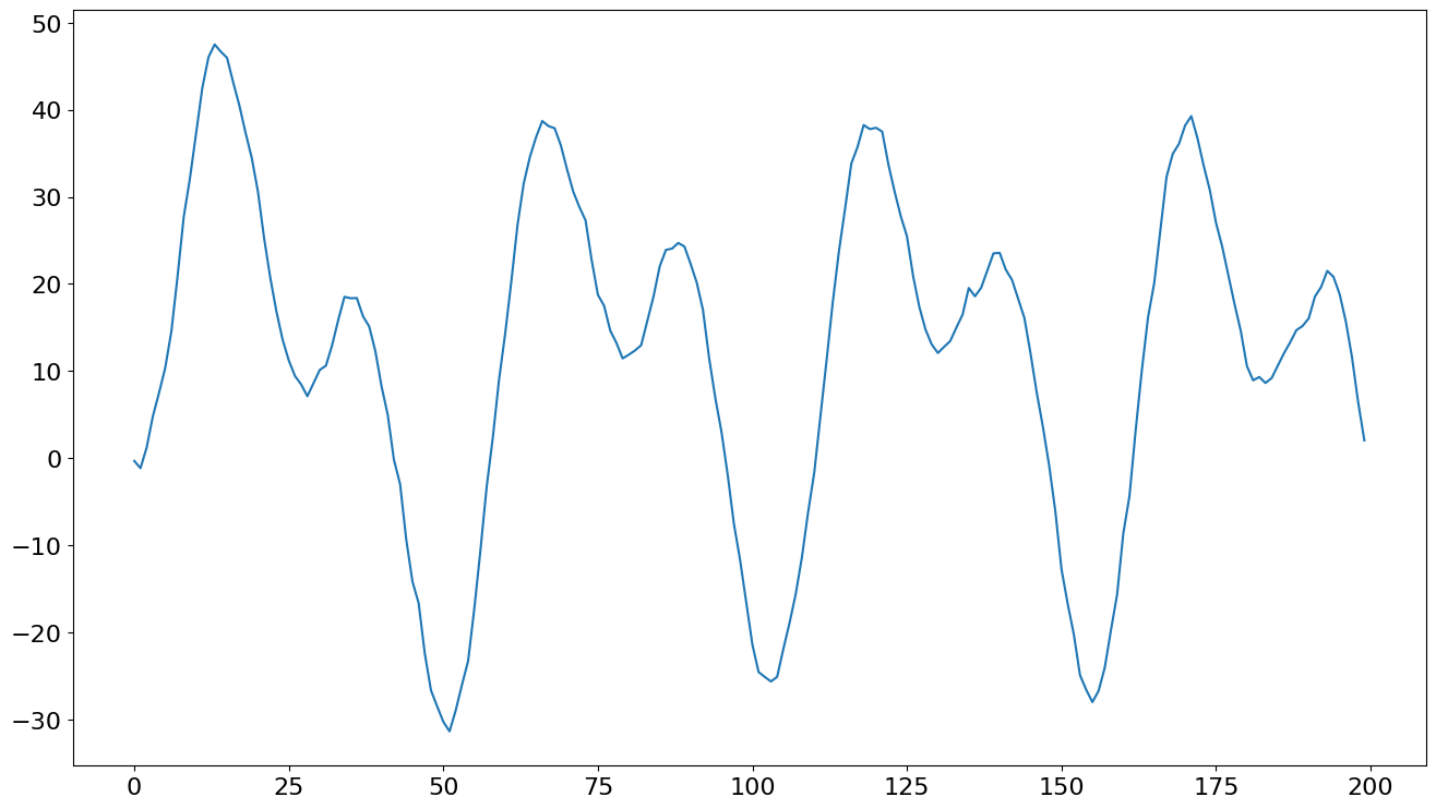
在這裡,我們模擬一些資料,這些資料具有傅立葉級數捕捉的每週季節性。
[17]:
gen = np.random.default_rng(98765432101234567890)
idx = pd.RangeIndex(200)
det_proc = DeterministicProcess(idx, constant=True, period=52, fourier=2)
det_terms = det_proc.in_sample().to_numpy()
params = np.array([1.0, 3, -1, 4, -2])
exog = det_terms @ params
y = np.empty(200)
y[0] = det_terms[0] @ params + gen.standard_normal()
for i in range(1, 200):
    y[i] = 0.9 * y[i - 1] + det_terms[i] @ params + gen.standard_normal()
y = pd.Series(y, index=idx)
ax = y.plot()
然後,使用 deterministic 關鍵字引數擬合模型。seasonal 預設為 False,但 trend 預設為 "c",因此需要變更。
[18]:
from statsmodels.tsa.api import AutoReg

mod = AutoReg(y, 1, trend="n", deterministic=det_proc)
res = mod.fit()
print(res.summary())
                            AutoReg Model Results
==============================================================================
Dep. Variable:                      y   No. Observations:                  200
Model:                     AutoReg(1)   Log Likelihood                -270.964
Method:               Conditional MLE   S.D. of innovations              0.944
Date:                Thu, 03 Oct 2024   AIC                            555.927
Time:                        15:46:43   BIC                            578.980
Sample:                             1   HQIC                           565.258
                                  200
==============================================================================
                 coef    std err          z      P>|z|      [0.025      0.975]
------------------------------------------------------------------------------
const          0.8436      0.172      4.916      0.000       0.507       1.180
sin(1,52)      2.9738      0.160     18.587      0.000       2.660       3.287
cos(1,52)     -0.6771      0.284     -2.380      0.017      -1.235      -0.120
sin(2,52)      3.9951      0.099     40.336      0.000       3.801       4.189
cos(2,52)     -1.7206      0.264     -6.519      0.000      -2.238      -1.203
y.L1           0.9116      0.014     63.264      0.000       0.883       0.940
                                    Roots
=============================================================================
                  Real          Imaginary           Modulus         Frequency
-----------------------------------------------------------------------------
AR.1            1.0970           +0.0000j            1.0970            0.0000
-----------------------------------------------------------------------------
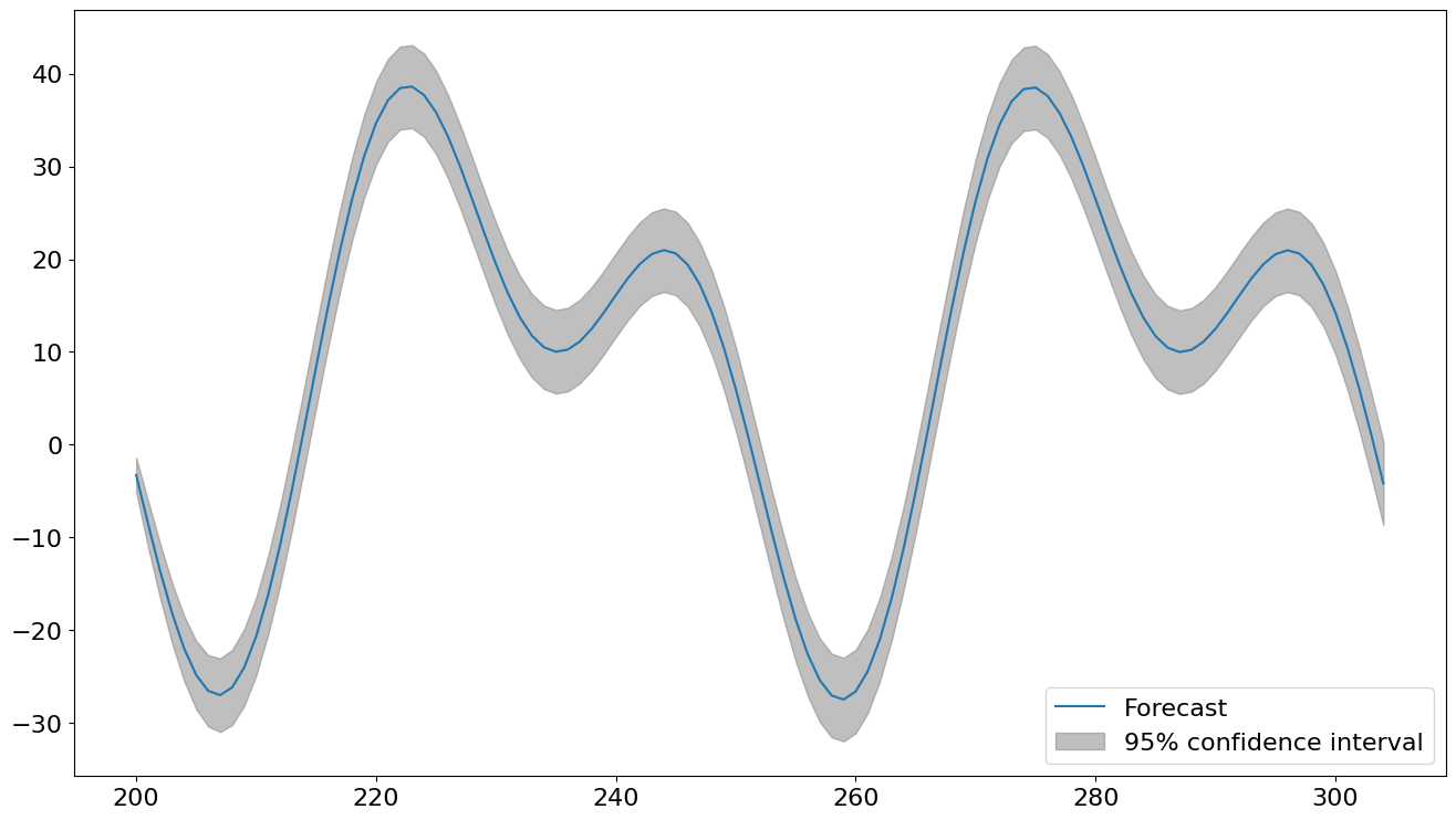
我們可以使用 plot_predict 來顯示預測值及其預測區間。樣本外確定性值會由傳遞給 AutoReg 的確定性過程自動產生。
[19]:
fig = res.plot_predict(200, 200 + 2 * 52, True)
[20]:
auto_reg_forecast = res.predict(200, 211)
auto_reg_forecast
[20]:
200    -3.253482
201    -8.555660
202   -13.607557
203   -18.152622
204   -21.950370
205   -24.790116
206   -26.503171
207   -26.972781
208   -26.141244
209   -24.013773
210   -20.658891
211   -16.205310
dtype: float64
與其他模型一起使用
其他模型不直接支援 DeterministicProcess。相反,我們可以手動將任何確定性項作為 exog 傳遞給支援外生值的模型。
請注意,具有外生變數的 SARIMAX 是具有 SARIMA 誤差的 OLS,因此模型為
確定性項的參數與 AutoReg 不直接可比較,AutoReg 依據以下方程式演變
當 \(x_t\) 僅包含確定性項時,這兩個表示形式是等效的(假設 \(\theta(L)=0\),因此沒有 MA)。
[21]:
from statsmodels.tsa.api import SARIMAX

det_proc = DeterministicProcess(idx, period=52, fourier=2)
det_terms = det_proc.in_sample()

mod = SARIMAX(y, order=(1, 0, 0), trend="c", exog=det_terms)
res = mod.fit(disp=False)
print(res.summary())
                               SARIMAX Results
==============================================================================
Dep. Variable:                      y   No. Observations:                  200
Model:               SARIMAX(1, 0, 0)   Log Likelihood                -293.381
Date:                Thu, 03 Oct 2024   AIC                            600.763
Time:                        15:46:44   BIC                            623.851
Sample:                             0   HQIC                           610.106
                                - 200
Covariance Type:                  opg
==============================================================================
                 coef    std err          z      P>|z|      [0.025      0.975]
------------------------------------------------------------------------------
intercept      0.0796      0.140      0.567      0.571      -0.196       0.355
sin(1,52)      9.1917      0.876     10.492      0.000       7.475      10.909
cos(1,52)    -17.4351      0.891    -19.576      0.000     -19.181     -15.689
sin(2,52)      1.2509      0.466      2.683      0.007       0.337       2.165
cos(2,52)    -17.1865      0.434    -39.582      0.000     -18.038     -16.335
ar.L1          0.9957      0.007    150.751      0.000       0.983       1.009
sigma2         1.0748      0.119      9.067      0.000       0.842       1.307
===================================================================================
Ljung-Box (L1) (Q):                   2.16   Jarque-Bera (JB):                 1.03
Prob(Q):                              0.14   Prob(JB):                         0.60
Heteroskedasticity (H):               0.71   Skew:                            -0.14
Prob(H) (two-sided):                  0.16   Kurtosis:                         2.78
===================================================================================

Warnings:
[1] Covariance matrix calculated using the outer product of gradients (complex-step).
預測相似,但因 SARIMAX 的參數是使用 MLE 估計的,而 AutoReg 使用 OLS,因此預測會有所不同。
[22]:
sarimax_forecast = res.forecast(12, exog=det_proc.out_of_sample(12))
df = pd.concat([auto_reg_forecast, sarimax_forecast], axis=1)
df.columns = columns = ["AutoReg", "SARIMAX"]
df
[22]:
| AutoReg | SARIMAX | |
|---|---|---|
| 200 | -3.253482 | -2.956589 |
| 201 | -8.555660 | -7.985653 |
| 202 | -13.607557 | -12.794185 |
| 203 | -18.152622 | -17.131131 |
| 204 | -21.950370 | -20.760701 |
| 205 | -24.790116 | -23.475800 |
| 206 | -26.503171 | -25.109977 |
| 207 | -26.972781 | -25.547191 |
| 208 | -26.141244 | -24.728829 |
| 209 | -24.013773 | -22.657570 |
| 210 | -20.658891 | -19.397843 |
| 211 | -16.205310 | -15.072875 |