使用局部加權迴歸 (LOESS) 的多重季節趨勢分解 (MSTL)¶

此筆記本說明如何使用 MSTL [1] 將時間序列分解為：趨勢成分、多個季節成分和殘差成分。MSTL 使用 STL（使用 LOESS 的季節趨勢分解）從時間序列迭代提取季節成分。MSTL 的關鍵輸入是

periods - 每個季節成分的週期（例如，對於具有每日和每週季節性的小時數據，我們會有：periods=(24, 24*7)）。
windows - 每個季節平滑器相對於每個週期的長度。如果這些值很大，則季節成分隨著時間的推移將顯示較小的變異性。必須為奇數。如果為 None，則使用原始論文 [1] 中實驗確定的一組預設值。
lmbda - 在分解之前進行 Box-Cox 轉換的 lambda 參數。如果為 None，則不進行轉換。如果為 "auto"，則會從資料中自動選擇適當的 lambda 值。
iterate - 用於精煉季節成分的迭代次數。
stl_kwargs - 所有可以傳遞給 STL 的其他參數（例如，robust、seasonal_deg 等）。請參閱 STL 文件。

[1] K. Bandura、R.J. Hyndman 和 C. Bergmeir (2021) MSTL：一種用於具有多重季節模式的時間序列的季節趨勢分解演算法。arXiv 預印本 arXiv:2107.13462。

請注意，此實作與 1 有一些關鍵差異。遺失的資料必須在 MSTL 類別之外處理。論文中提出的演算法會處理沒有季節性的情況。此實作假設至少有一個季節成分。

首先，我們導入所需的套件、準備圖形環境並準備資料。

[1]:

import matplotlib.pyplot as plt
import datetime
import pandas as pd
import numpy as np
import seaborn as sns
from pandas.plotting import register_matplotlib_converters

from statsmodels.tsa.seasonal import MSTL
from statsmodels.tsa.seasonal import DecomposeResult

register_matplotlib_converters()
sns.set_style("darkgrid")

[2]:

plt.rc("figure", figsize=(16, 12))
plt.rc("font", size=13)

MSTL 應用於玩具資料集¶

建立具有多重季節性的玩具資料集¶

我們建立一個具有小時頻率的時間序列，其中具有每日和每週季節性，且遵循正弦波。我們將在本筆記本的稍後部分示範一個更真實的範例。

[3]:

t = np.arange(1, 1000)
daily_seasonality = 5 * np.sin(2 * np.pi * t / 24)
weekly_seasonality = 10 * np.sin(2 * np.pi * t / (24 * 7))
trend = 0.0001 * t**2
y = trend + daily_seasonality + weekly_seasonality + np.random.randn(len(t))
ts = pd.date_range(start="2020-01-01", freq="H", periods=len(t))
df = pd.DataFrame(data=y, index=ts, columns=["y"])

/tmp/ipykernel_5245/288299940.py:6: FutureWarning: 'H' is deprecated and will be removed in a future version, please use 'h' instead.
  ts = pd.date_range(start="2020-01-01", freq="H", periods=len(t))

[4]:

df.head()

[4]:

	y
2020-01-01 00:00:00	2.430365
2020-01-01 01:00:00	1.790566
2020-01-01 02:00:00	4.625017
2020-01-01 03:00:00	7.025365
2020-01-01 04:00:00	7.388021

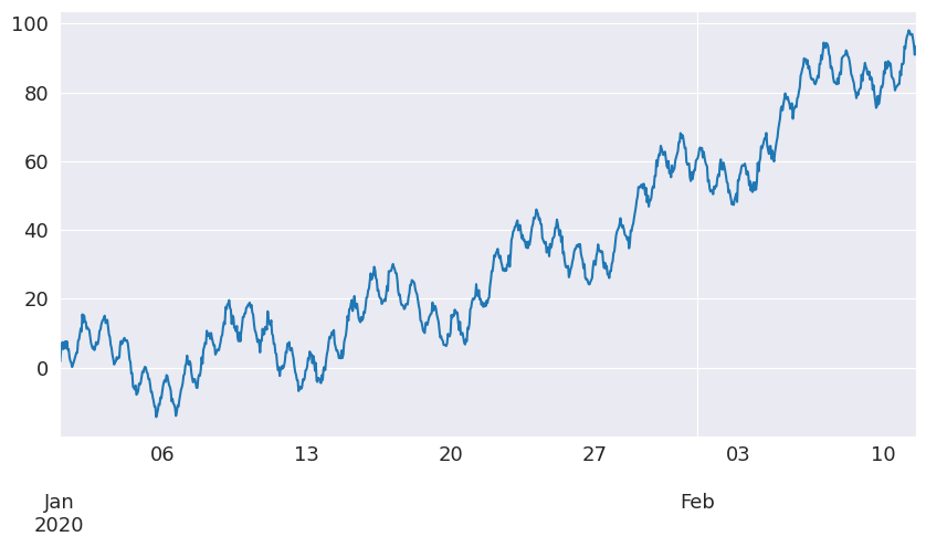
讓我們繪製時間序列

[5]:

df["y"].plot(figsize=[10, 5])

[5]:

<Axes: >

../../../_images/examples_notebooks_generated_mstl_decomposition_9_1.png

使用 MSTL 分解玩具資料集¶

讓我們使用 MSTL 將時間序列分解為趨勢成分、每日和每週季節成分以及殘差成分。

[6]:

mstl = MSTL(df["y"], periods=[24, 24 * 7])
res = mstl.fit()

如果輸入是 pandas 資料框架，則季節成分的輸出為資料框架。每個成分的週期都反映在欄名稱中。

[7]:

res.seasonal.head()

[7]:

	seasonal_24	seasonal_168
2020-01-01 00:00:00	1.500231	1.796102
2020-01-01 01:00:00	2.339523	0.227047
2020-01-01 02:00:00	2.736665	2.076791
2020-01-01 03:00:00	5.812639	1.220039
2020-01-01 04:00:00	4.672422	3.259005

[8]:

ax = res.plot()

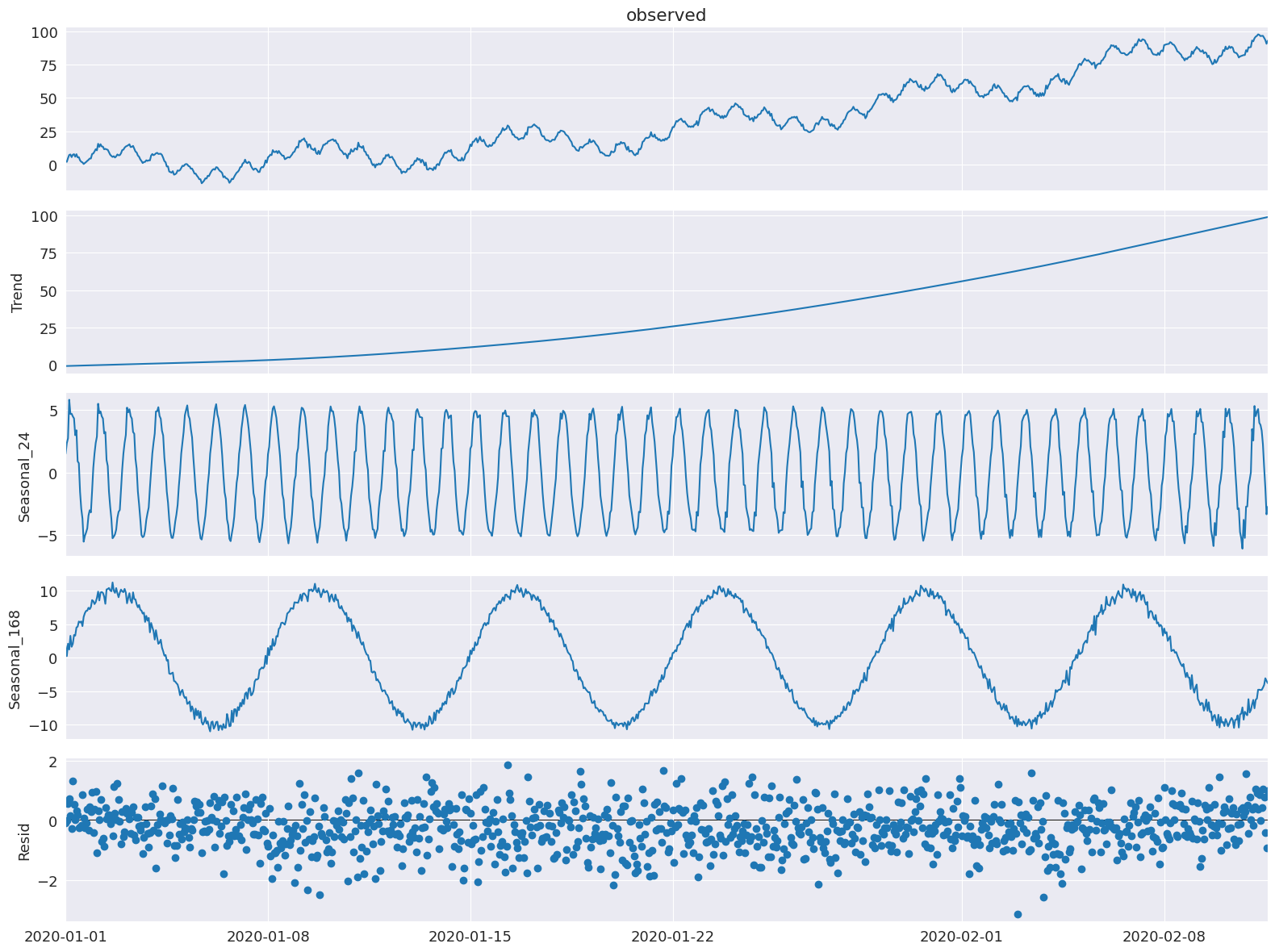
../../../_images/examples_notebooks_generated_mstl_decomposition_15_0.png

我們看到每小時和每週的季節成分已被提取。

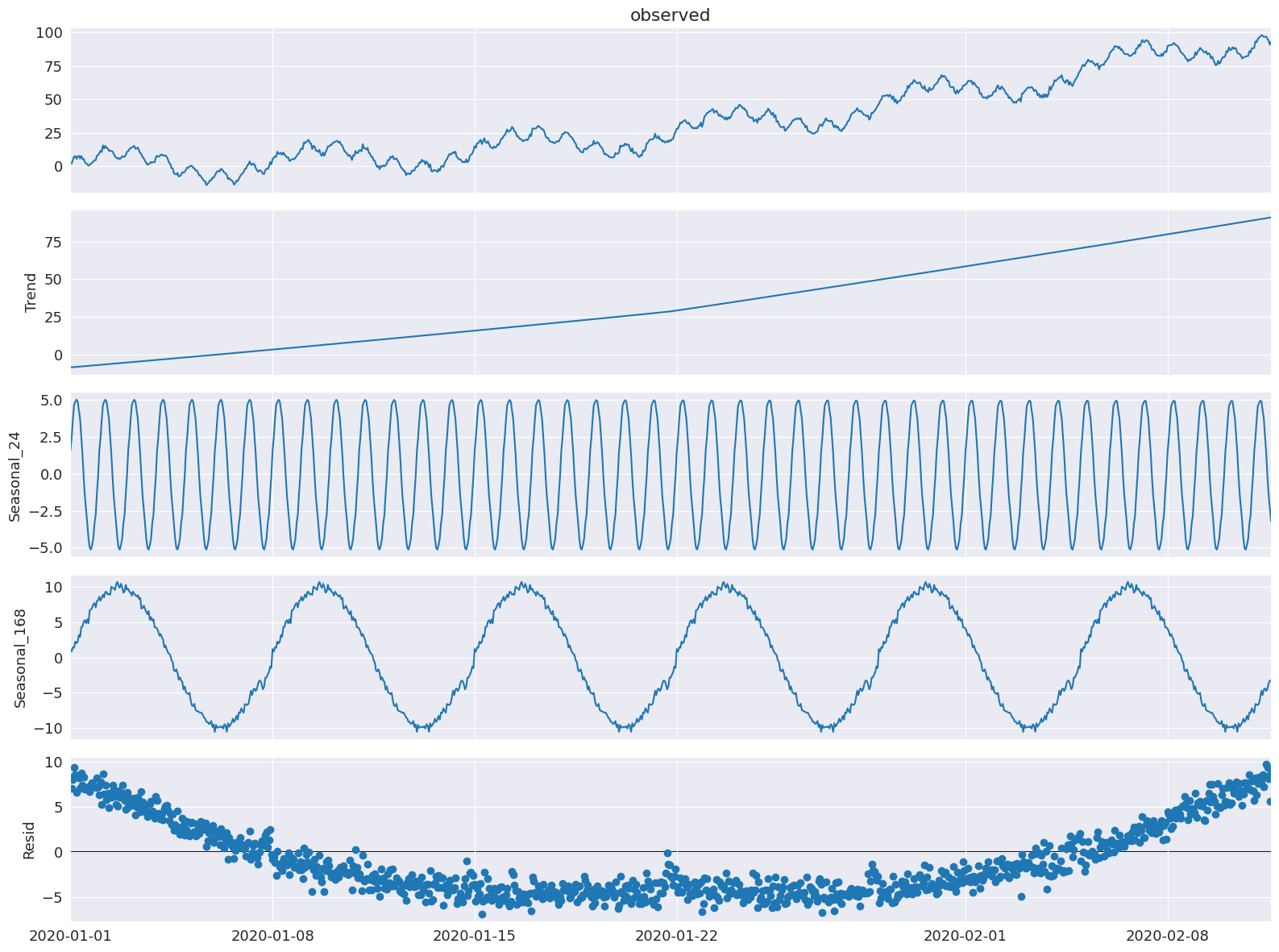
除了 period 和 seasonal 之外的任何 STL 參數（因為它們由 MSTL 中的 periods 和 windows 設定）也可以透過將 arg:value 對作為字典傳遞給 stl_kwargs 來設定（我們現在將在一個範例中展示）。

在這裡，我們展示了我們仍然可以透過 trend 設定 STL 的趨勢平滑器，並透過 seasonal_deg 設定季節擬合的多項式階數。我們還將明確設定 windows、seasonal_deg 和 iterate 參數。我們將獲得更差的擬合，但這僅是如何將這些參數傳遞給 MSTL 類別的範例。

[9]:

mstl = MSTL(
    df,
    periods=[24, 24 * 7],  # The periods and windows must be the same length and will correspond to one another.
    windows=[101, 101],  # Setting this large along with `seasonal_deg=0` will force the seasonality to be periodic.
    iterate=3,
    stl_kwargs={
                "trend":1001, # Setting this large will force the trend to be smoother.
                "seasonal_deg":0, # Means the seasonal smoother is fit with a moving average.
               }
)
res = mstl.fit()
ax = res.plot()

../../../_images/examples_notebooks_generated_mstl_decomposition_18_0.png

MSTL 應用於電力需求資料集¶

準備資料¶

我們將使用此處找到的維多利亞電力需求資料集：https://github.com/tidyverts/tsibbledata/tree/master/data-raw/vic_elec。此資料集用於原始 MSTL 論文 [1] 中。它是澳洲維多利亞州從 2002 年到 2015 年初的半小時粒度總電力需求。有關該資料集的更詳細描述，請參閱此處。

[10]:

url = "https://raw.githubusercontent.com/tidyverts/tsibbledata/master/data-raw/vic_elec/VIC2015/demand.csv"
df = pd.read_csv(url)

[11]:

df.head()

[11]:

	日期	週期	營運減去工業	工業
0	37257	1	3535.867064	1086.132936
1	37257	2	3383.499028	1088.500972
2	37257	3	3655.527552	1084.472448
3	37257	4	3510.446636	1085.553364
4	37257	5	3294.697156	1081.302844

日期是表示自起始日期以來天數的整數。此資料集的起始日期由此處和此處決定，為「1899-12-30」。週期 整數是指 24 小時內 30 分鐘的間隔，因此每天有 48 個。

讓我們提取日期和日期時間。

[12]:

df["Date"] = df["Date"].apply(lambda x: pd.Timestamp("1899-12-30") + pd.Timedelta(x, unit="days"))
df["ds"] = df["Date"] + pd.to_timedelta((df["Period"]-1)*30, unit="m")

我們將對 OperationalLessIndustrial 感興趣，它是排除某些高能量工業使用者的需求的電力需求。我們將把資料重新取樣為每小時，並將資料篩選為與原始 MSTL 論文 [1] 相同的時間段，也就是 2012 年的前 149 天。

[13]:

timeseries = df[["ds", "OperationalLessIndustrial"]]
timeseries.columns = ["ds", "y"] # Rename to OperationalLessIndustrial to y for simplicity.

# Filter for first 149 days of 2012.
start_date = pd.to_datetime("2012-01-01")
end_date = start_date + pd.Timedelta("149D")
mask = (timeseries["ds"] >= start_date) & (timeseries["ds"] < end_date)
timeseries = timeseries[mask]

# Resample to hourly
timeseries = timeseries.set_index("ds").resample("H").sum()
timeseries.head()

/tmp/ipykernel_5245/185151541.py:11: FutureWarning: 'H' is deprecated and will be removed in a future version, please use 'h' instead.
  timeseries = timeseries.set_index("ds").resample("H").sum()

[13]:

	y
ds
2012-01-01 00:00:00	7926.529376
2012-01-01 01:00:00	7901.826990
2012-01-01 02:00:00	7255.721350
2012-01-01 03:00:00	6792.503352
2012-01-01 04:00:00	6635.984460

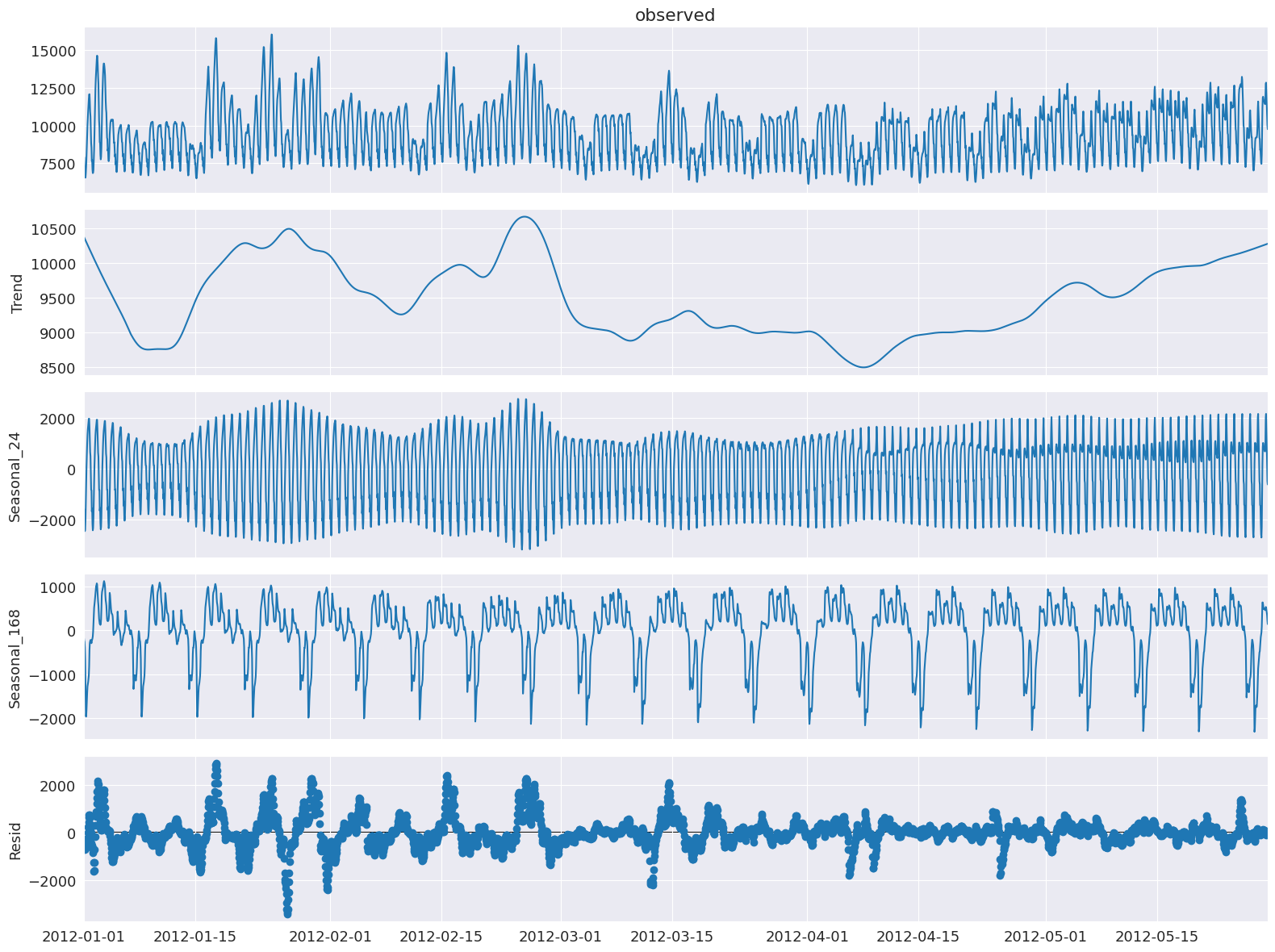
使用 MSTL 分解電力需求¶

讓我們將 MSTL 應用於此資料集。

注意：stl_kwargs 設定為給出與 [1] 接近的結果，該論文使用了 R，因此對於底層 STL 參數具有稍微不同的預設設定。在實務上，很少會手動明確設定 inner_iter 和 outer_iter。

[14]:

mstl = MSTL(timeseries["y"], periods=[24, 24 * 7], iterate=3, stl_kwargs={"seasonal_deg": 0,
                                                                          "inner_iter": 2,
                                                                          "outer_iter": 0})
res = mstl.fit() # Use .fit() to perform and return the decomposition
ax = res.plot()
plt.tight_layout()

../../../_images/examples_notebooks_generated_mstl_decomposition_30_0.png

多個季節成分以 pandas 資料框架的形式儲存在 seasonal 屬性中

[15]:

res.seasonal.head()

[15]:

	seasonal_24	seasonal_168
ds
2012-01-01 00:00:00	-1685.986297	-161.807086
2012-01-01 01:00:00	-1591.640845	-229.788887
2012-01-01 02:00:00	-2192.989492	-260.121300
2012-01-01 03:00:00	-2442.169359	-388.484499
2012-01-01 04:00:00	-2357.492551	-660.245476

讓我們更詳細地檢查季節成分，並查看前幾天和幾週，以檢查每日和每週的季節性。

[16]:

fig, ax = plt.subplots(nrows=2, figsize=[10,10])
res.seasonal["seasonal_24"].iloc[:24*3].plot(ax=ax[0])
ax[0].set_ylabel("seasonal_24")
ax[0].set_title("Daily seasonality")

res.seasonal["seasonal_168"].iloc[:24*7*3].plot(ax=ax[1])
ax[1].set_ylabel("seasonal_168")
ax[1].set_title("Weekly seasonality")

plt.tight_layout()

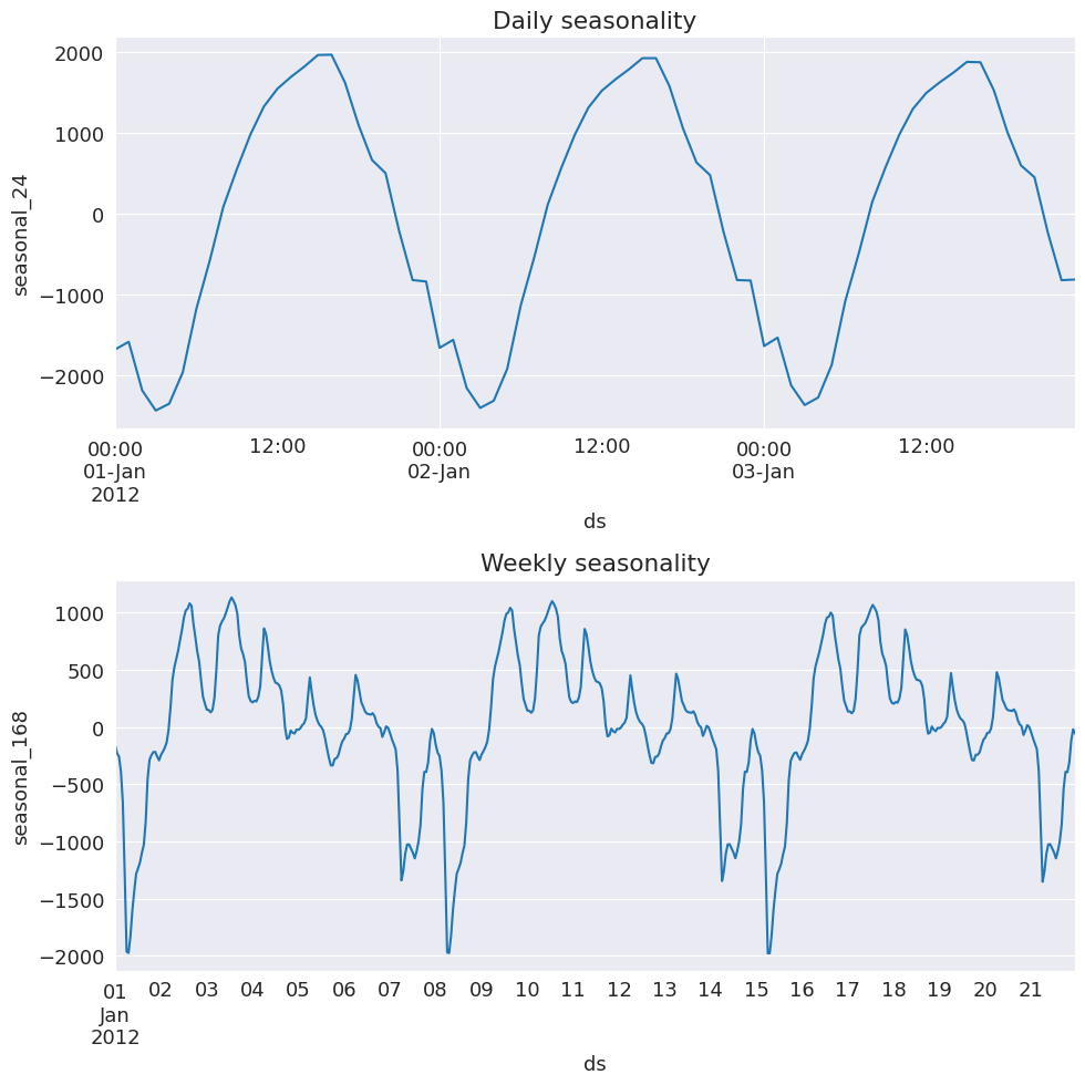
../../../_images/examples_notebooks_generated_mstl_decomposition_34_0.png

我們可以看到電力需求的每日季節性已被很好地捕捉。這是一月份的前幾天，因此在澳洲的夏季，下午會出現高峰，很可能是由於空調的使用。

對於每週季節性，我們可以看到週末的使用量較少。

MSTL 的優勢之一是它可以讓我們捕捉到隨時間變化的季節性。因此，讓我們看看五月份較冷月份的季節性。

[17]:

fig, ax = plt.subplots(nrows=2, figsize=[10,10])
mask = res.seasonal.index.month==5
res.seasonal[mask]["seasonal_24"].iloc[:24*3].plot(ax=ax[0])
ax[0].set_ylabel("seasonal_24")
ax[0].set_title("Daily seasonality")

res.seasonal[mask]["seasonal_168"].iloc[:24*7*3].plot(ax=ax[1])
ax[1].set_ylabel("seasonal_168")
ax[1].set_title("Weekly seasonality")

plt.tight_layout()

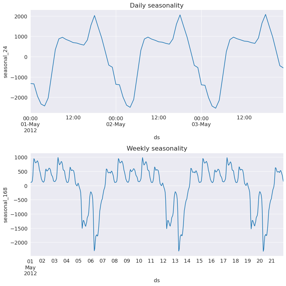
../../../_images/examples_notebooks_generated_mstl_decomposition_36_0.png

現在我們可以看見傍晚的額外高峰！這可能與傍晚需要的暖氣和照明有關。所以這說得通。我們看到週末需求量較低的主要每週模式持續存在。

其他成分也可以從 trend 和 resid 屬性中提取

[18]:

display(res.trend.head()) # trend component
display(res.resid.head()) # residual component

ds
2012-01-01 00:00:00    10373.942662
2012-01-01 01:00:00    10363.488489
2012-01-01 02:00:00    10353.037721
2012-01-01 03:00:00    10342.590527
2012-01-01 04:00:00    10332.147100
Freq: h, Name: trend, dtype: float64

ds
2012-01-01 00:00:00   -599.619903
2012-01-01 01:00:00   -640.231767
2012-01-01 02:00:00   -644.205579
2012-01-01 03:00:00   -719.433316
2012-01-01 04:00:00   -678.424613
Freq: h, Name: resid, dtype: float64

就是這樣！使用 MSTL，我們可以在多季節時間序列上執行時間序列分解！

上次更新：2024 年 10 月 3 日