使用 LOESS 的季節性趨勢分解 (STL)¶

本筆記本說明如何使用 STL 將時間序列分解為三個組成部分：趨勢、季節性（或季節）和殘差。STL 使用 LOESS（局部加權散佈圖平滑）來提取三個組成部分的平滑估計值。STL 的主要輸入是

season - 季節性平滑器的長度。必須為奇數。
trend - 趨勢平滑器的長度，通常約為 season 的 150%。必須為奇數且大於 season。
low_pass - 低通估計視窗的長度，通常是比數據週期性大的最小奇數。

首先，我們匯入所需的套件，準備圖形環境，並準備數據。

[1]:

import matplotlib.pyplot as plt
import pandas as pd
import seaborn as sns
from pandas.plotting import register_matplotlib_converters

register_matplotlib_converters()
sns.set_style("darkgrid")

[2]:

plt.rc("figure", figsize=(16, 12))
plt.rc("font", size=13)

大氣中的二氧化碳¶

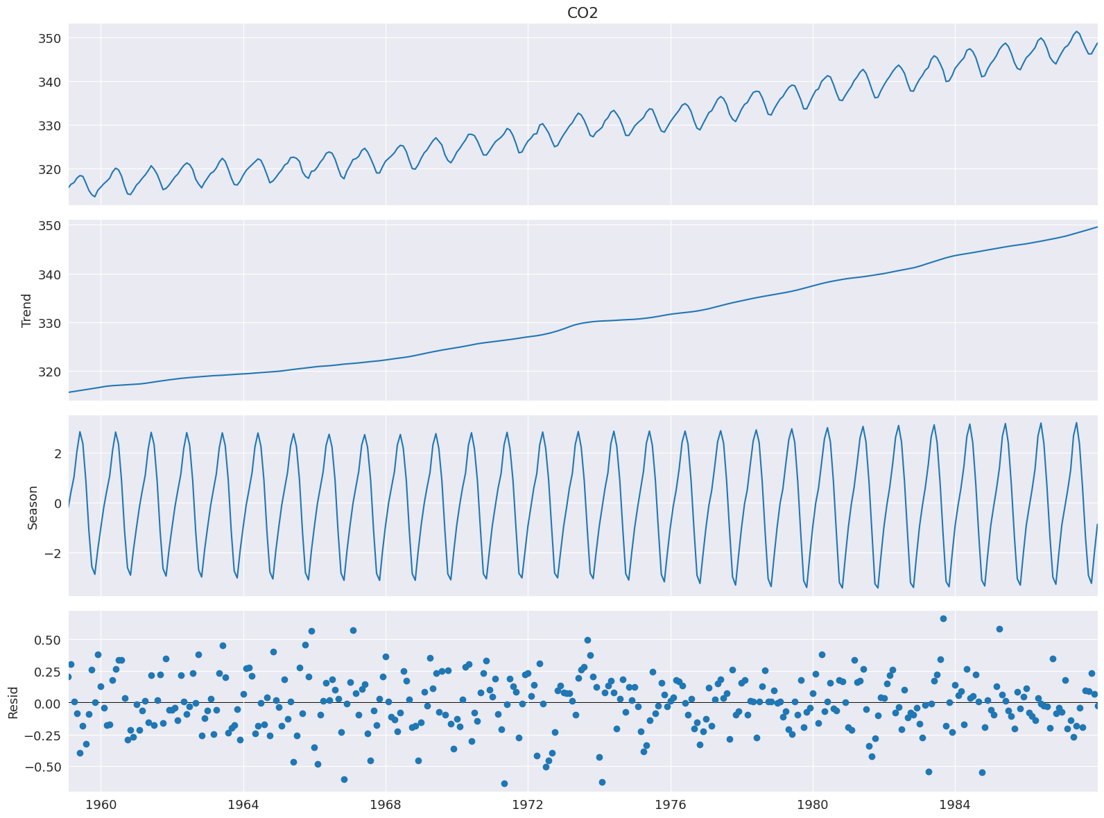
Cleveland, Cleveland, McRae 和 Terpenning (1990) 中的範例使用二氧化碳數據，該數據在下面的列表中。這個每月數據（1959 年 1 月至 1987 年 12 月）在整個樣本中具有明顯的趨勢和季節性。

[3]:

co2 = [
58,
39,
79,
82,
39,
22,
68,
01,
02,
55,
02,
75,
52,
10,
79,
22,
08,
70,
27,
99,
24,
05,
05,
23,
92,
76,
54,
49,
64,
85,
70,
96,
17,
47,
19,
17,
12,
72,
79,
68,
28,
89,
79,
56,
46,
59,
85,
87,
87,
25,
13,
49,
34,
62,
85,
87,
36,
24,
13,
46,
57,
23,
89,
54,
20,
90,
42,
60,
73,
15,
94,
91,
73,
78,
23,
49,
59,
35,
61,
24,
23,
76,
36,
50,
35,
40,
22,
45,
80,
50,
16,
09,
26,
66,
47,
70,
06,
23,
78,
10,
63,
79,
34,
73,
00,
99,
41,
68,
30,
89,
59,
65,
30,
15,
88,
80,
99,
86,
88,
36,
59,
23,
34,
33,
03,
24,
39,
16,
87,
31,
34,
74,
61,
58,
55,
81,
82,
53,
29,
66,
12,
09,
01,
10,
12,
62,
16,
94,
15,
79,
53,
65,
60,
78,
13,
26,
93,
84,
96,
93,
25,
24,
13,
42,
97,
29,
56,
73,
73,
70,
46,
70,
66,
22,
02,
39,
58,
27,
30,
81,
44,
89,
62,
85,
29,
44,
35,
58,
58,
55,
56,
73,
45,
98,
63,
88,
63,
53,
90,
08,
59,
31,
44,
64,
62,
45,
36,
46,
84,
29,
04,
88,
23,
83,
18,
50,
80,
22,
54,
82,
45,
97,
65,
40,
28,
73,
05,
54,
65,
06,
32,
39,
66,
56,
24,
39,
43,
22,
61,
78,
88,
43,
61,
53,
06,
92,
39,
72,
64,
65,
07,
53,
82,
19,
89,
56,
22,
92,
26,
27,
66,
54,
71,
79,
79,
06,
93,
02,
65,
80,
01,
94,
17,
28,
76,
05,
18,
04,
16,
01,
64,
91,
72,
52,
75,
68,
14,
37,
32,
45,
05,
91,
77,
30,
98,
41,
89,
03,
19,
87,
74,
55,
28,
00,
37,
74,
36,
19,
97,
20,
76,
96,
82,
82,
24,
09,
66,
90,
27,
21,
88,
58,
99,
31,
98,
72,
63,
24,
83,
10,
52,
43,
48,
89,
29,
54,
66,
07,
12,
55,
34,
80,
10,
54,
20,
20,
44,
67,
]
co2 = pd.Series(
    co2, index=pd.date_range("1-1-1959", periods=len(co2), freq="M"), name="CO2"
)
co2.describe()

/tmp/ipykernel_3881/1071343913.py:352: FutureWarning: 'M' is deprecated and will be removed in a future version, please use 'ME' instead.
  co2, index=pd.date_range("1-1-1959", periods=len(co2), freq="M"), name="CO2"

[3]:

count    348.000000
mean     330.123879
std       10.059747
min      313.550000
25%      321.302500
50%      328.820000
75%      338.002500
max      351.340000
Name: CO2, dtype: float64

分解需要 1 個輸入，即數據序列。如果數據序列沒有頻率，則還必須指定 period。seasonal 的預設值為 7，因此在大多數應用中也應更改。

[4]:

from statsmodels.tsa.seasonal import STL

stl = STL(co2, seasonal=13)
res = stl.fit()
fig = res.plot()

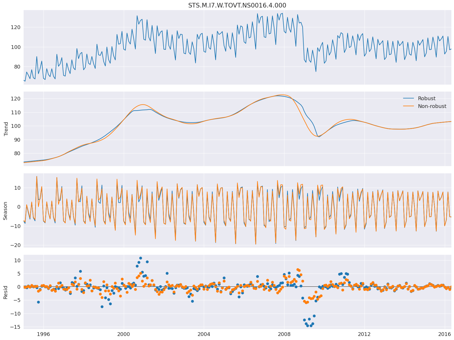
../../../_images/examples_notebooks_generated_stl_decomposition_6_0.png

穩健擬合¶

設定 robust 會使用與數據相關的加權函數，在估計 LOESS 時重新加權數據（因此使用 LOWESS）。使用穩健估計可以讓模型容忍底部圖中可見的較大誤差。

在這裡，我們使用一個衡量歐盟電氣設備產量的序列。

[5]:

from statsmodels.datasets import elec_equip as ds

elec_equip = ds.load().data.iloc[:, 0]

接下來，我們估計有和沒有穩健加權的模型。差異很小，在 2008 年的金融危機期間最為明顯。非穩健估計會對所有觀測值給予相同的權重，因此平均會產生較小的誤差。權重在 0 和 1 之間變化。

[6]:

def add_stl_plot(fig, res, legend):
    """Add 3 plots from a second STL fit"""
    axs = fig.get_axes()
    comps = ["trend", "seasonal", "resid"]
    for ax, comp in zip(axs[1:], comps):
        series = getattr(res, comp)
        if comp == "resid":
            ax.plot(series, marker="o", linestyle="none")
        else:
            ax.plot(series)
            if comp == "trend":
                ax.legend(legend, frameon=False)

stl = STL(elec_equip, period=12, robust=True)
res_robust = stl.fit()
fig = res_robust.plot()
res_non_robust = STL(elec_equip, period=12, robust=False).fit()
add_stl_plot(fig, res_non_robust, ["Robust", "Non-robust"])

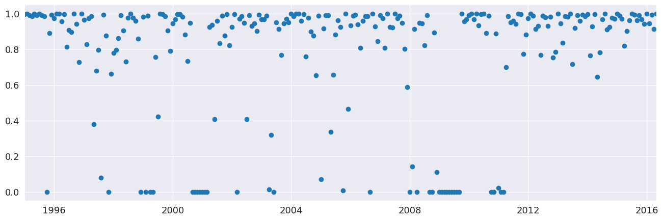
../../../_images/examples_notebooks_generated_stl_decomposition_10_0.png

[7]:

fig = plt.figure(figsize=(16, 5))
lines = plt.plot(res_robust.weights, marker="o", linestyle="none")
ax = plt.gca()
xlim = ax.set_xlim(elec_equip.index[0], elec_equip.index[-1])

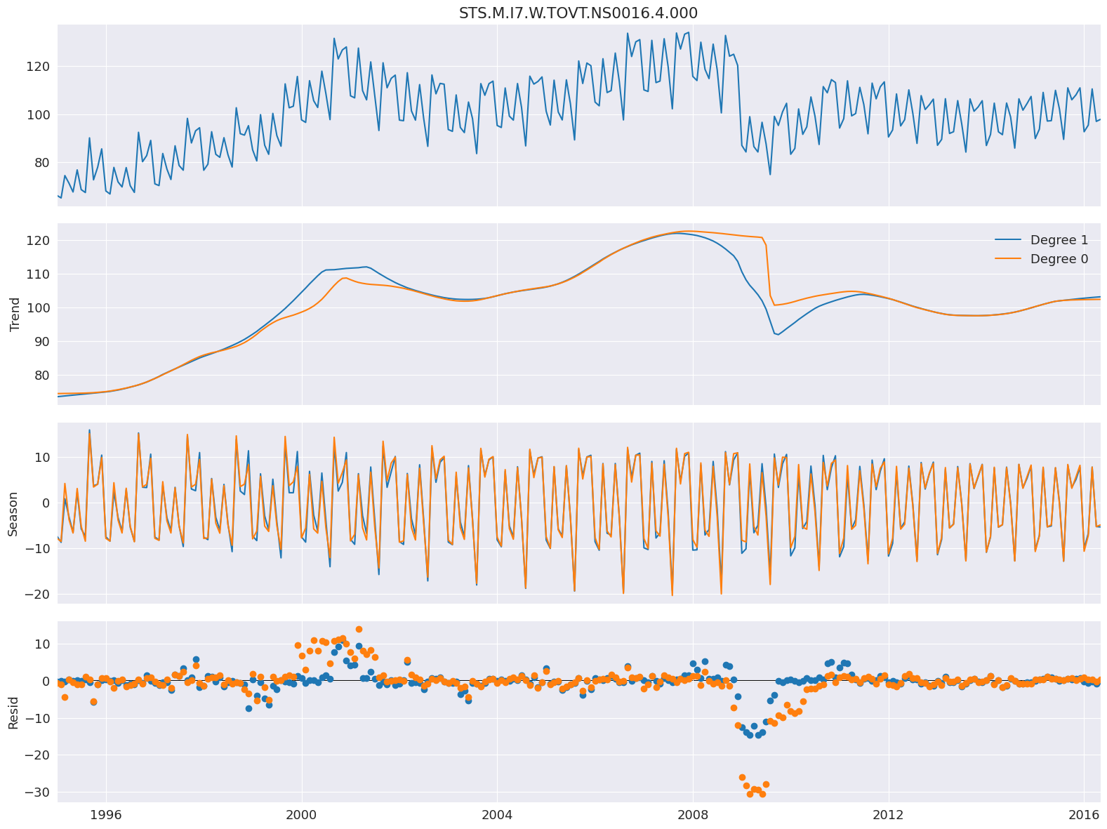
../../../_images/examples_notebooks_generated_stl_decomposition_11_0.png

LOESS 次數¶

預設設定會使用常數和趨勢估計 LOESS 模型。可以將其更改為僅包含常數，方法是將 COMPONENT_deg 設定為 0。這裡的次數除了在 2008 年金融危機附近的趨勢之外，幾乎沒有差別。

[8]:

stl = STL(
    elec_equip, period=12, seasonal_deg=0, trend_deg=0, low_pass_deg=0, robust=True
)
res_deg_0 = stl.fit()
fig = res_robust.plot()
add_stl_plot(fig, res_deg_0, ["Degree 1", "Degree 0"])

../../../_images/examples_notebooks_generated_stl_decomposition_13_0.png

效能¶

可以使用三個選項來降低 STL 分解的計算成本

seasonal_jump
trend_jump
low_pass_jump

當這些值不為零時，僅在每 COMPONENT_jump 個觀測值處估計成分 COMPONENT 的 LOESS，並且在點之間使用線性內插。這些值通常不應超過 seasonal、trend 或 low_pass 大小的 10-20%。

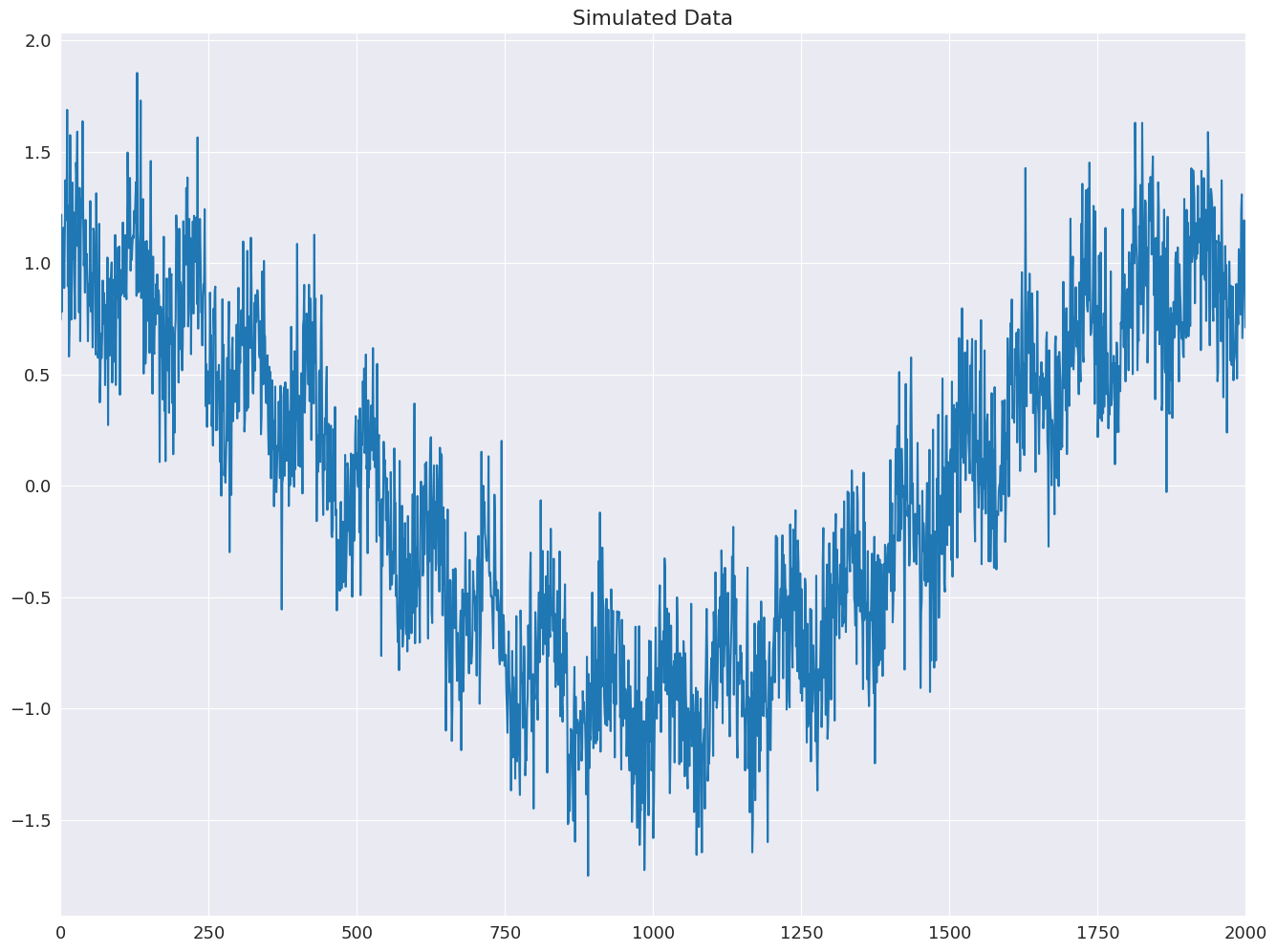
下面的範例顯示如何使用具有低頻餘弦趨勢和正弦季節性模式的模擬數據，將計算成本降低 15 倍。

[9]:

import numpy as np

rs = np.random.RandomState(0xA4FD94BC)
tau = 2000
t = np.arange(tau)
period = int(0.05 * tau)
seasonal = period + ((period % 2) == 0)  # Ensure odd
e = 0.25 * rs.standard_normal(tau)
y = np.cos(t / tau * 2 * np.pi) + 0.25 * np.sin(t / period * 2 * np.pi) + e
plt.plot(y)
plt.title("Simulated Data")
xlim = plt.gca().set_xlim(0, tau)

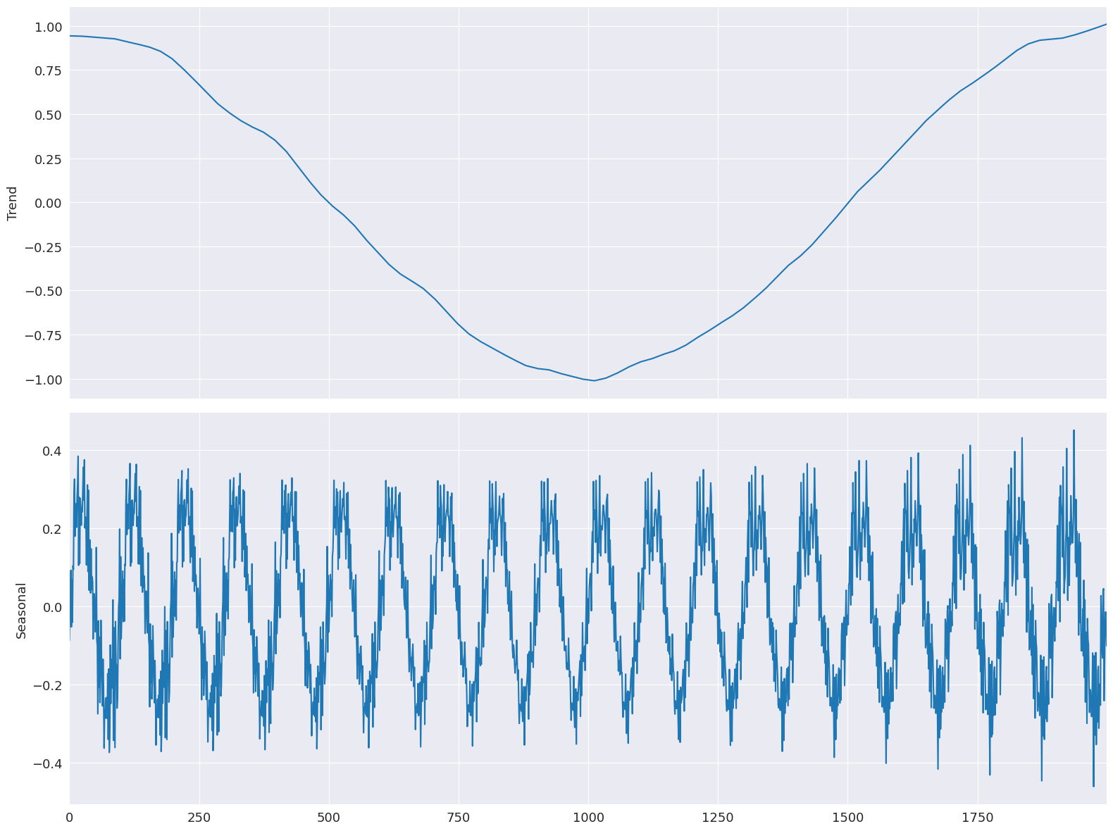
../../../_images/examples_notebooks_generated_stl_decomposition_15_0.png

首先，估計所有跳躍都等於 1 的基準模型。

[10]:

mod = STL(y, period=period, seasonal=seasonal)
%timeit mod.fit()
res = mod.fit()
fig = res.plot(observed=False, resid=False)

284 ms ± 38.9 ms per loop (mean ± std. dev. of 7 runs, 1 loop each)

../../../_images/examples_notebooks_generated_stl_decomposition_17_1.png

跳躍全部設定為其視窗長度的 15%。有限的線性內插對模型的擬合影響不大。

[11]:

low_pass_jump = seasonal_jump = int(0.15 * (period + 1))
trend_jump = int(0.15 * 1.5 * (period + 1))
mod = STL(
    y,
    period=period,
    seasonal=seasonal,
    seasonal_jump=seasonal_jump,
    trend_jump=trend_jump,
    low_pass_jump=low_pass_jump,
)
%timeit mod.fit()
res = mod.fit()
fig = res.plot(observed=False, resid=False)

22.9 ms ± 1.04 ms per loop (mean ± std. dev. of 7 runs, 10 loops each)

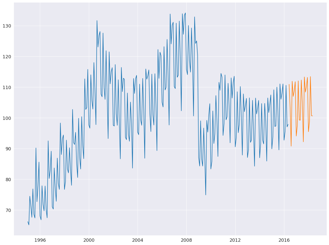
../../../_images/examples_notebooks_generated_stl_decomposition_19_1.png

使用 STL 進行預測¶

STLForecast 簡化了使用 STL 移除季節性，然後使用標準時間序列模型預測趨勢和循環成分的過程。

在這裡，我們使用 STL 來處理季節性，然後使用 ARIMA(1,1,0) 來建模去除季節性的數據。季節性成分是從找到完整週期的位置預測的，其中

\[E[S_{T+h}|\mathcal{F}_T]=\hat{S}_{T-k}\]

其中 \(k= m - h + m \lfloor \frac{h-1}{m} \rfloor\)。預測會自動將季節性成分預測新增到 ARIMA 預測中。

[12]:

from statsmodels.tsa.arima.model import ARIMA
from statsmodels.tsa.forecasting.stl import STLForecast

elec_equip.index.freq = elec_equip.index.inferred_freq
stlf = STLForecast(elec_equip, ARIMA, model_kwargs=dict(order=(1, 1, 0), trend="t"))
stlf_res = stlf.fit()

forecast = stlf_res.forecast(24)
plt.plot(elec_equip)
plt.plot(forecast)
plt.show()

../../../_images/examples_notebooks_generated_stl_decomposition_21_0.png

summary 包含有關時間序列模型和 STL 分解的資訊。

[13]:

print(stlf_res.summary())

                    STL Decomposition and SARIMAX Results
==============================================================================
Dep. Variable:                      y   No. Observations:                  257
Model:                 ARIMA(1, 1, 0)   Log Likelihood                -522.434
Date:                Thu, 03 Oct 2024   AIC                           1050.868
Time:                        15:45:57   BIC                           1061.504
Sample:                    01-01-1995   HQIC                          1055.146
                         - 05-01-2016
Covariance Type:                  opg
==============================================================================
                 coef    std err          z      P>|z|      [0.025      0.975]
------------------------------------------------------------------------------
x1             0.1171      0.118      0.995      0.320      -0.113       0.348
ar.L1         -0.0435      0.049     -0.880      0.379      -0.140       0.053
sigma2         3.4682      0.188     18.406      0.000       3.099       3.837
===================================================================================
Ljung-Box (L1) (Q):                   0.01   Jarque-Bera (JB):               223.01
Prob(Q):                              0.92   Prob(JB):                         0.00
Heteroskedasticity (H):               0.33   Skew:                            -0.26
Prob(H) (two-sided):                  0.00   Kurtosis:                         7.54
                                STL Configuration
=================================================================================
Period:                            12       Trend Length:                      23
Seasonal:                           7       Trend deg:                          1
Seasonal deg:                       1       Trend jump:                         1
Seasonal jump:                      1       Low pass:                          13
Robust:                         False       Low pass deg:                       1
---------------------------------------------------------------------------------

Warnings:
[1] Covariance matrix calculated using the outer product of gradients (complex-step).

上次更新：2024 年 10 月 03 日