馬可夫轉換動態迴歸模型
此筆記本提供一個在 statsmodels 中使用馬可夫轉換模型的範例,以估計具有狀態變化的動態迴歸模型。它遵循 Stata 馬可夫轉換文檔中的範例,該文檔可在 http://www.stata.com/manuals14/tsmswitch.pdf 找到。
[1]:
%matplotlib inline

import numpy as np
import pandas as pd
import statsmodels.api as sm
import matplotlib.pyplot as plt

# NBER recessions
from pandas_datareader.data import DataReader
from datetime import datetime

usrec = DataReader(
    "USREC", "fred", start=datetime(1947, 1, 1), end=datetime(2013, 4, 1)
)
具有轉換截距的聯邦基金利率
第一個範例將聯邦基金利率建模為圍繞常數截距的雜訊,但截距在不同狀態下會發生變化。該模型很簡單:
其中 \(S_t \in \{0, 1\}\),且狀態轉換如下:
我們將透過最大似然法估計此模型的參數:\(p_{00}, p_{10}, \mu_0, \mu_1, \sigma^2\)。
此範例中使用的資料可在 https://www.stata-press.com/data/r14/usmacro 找到。
[2]:
# Get the federal funds rate data
from statsmodels.tsa.regime_switching.tests.test_markov_regression import fedfunds
dta_fedfunds = pd.Series(
fedfunds, index=pd.date_range("1954-07-01", "2010-10-01", freq="QS")
)
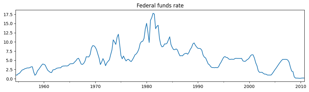
# Plot the data
dta_fedfunds.plot(title="Federal funds rate", figsize=(12, 3))
# Fit the model
# (a switching mean is the default of the MarkovRegession model)
mod_fedfunds = sm.tsa.MarkovRegression(dta_fedfunds, k_regimes=2)
res_fedfunds = mod_fedfunds.fit()
[3]:
res_fedfunds.summary()
[3]:
| 因變數 | y | 觀測數量 | 226 |
|---|---|---|---|
| 模型 | MarkovRegression | 對數概度 | -508.636 |
| 日期 | 週四, 2024年10月03日 | AIC | 1027.272 |
| 時間 | 15:45:37 | BIC | 1044.375 |
| 樣本 | 07-01-1954 | HQIC | 1034.174 |
| - 10-01-2010 | |||
| 共變異數類型 | 近似 |
| 係數 | 標準誤差 | z | P>|z| | [0.025 | 0.975] | |
|---|---|---|---|---|---|---|
| 常數 | 3.7088 | 0.177 | 20.988 | 0.000 | 3.362 | 4.055 |
| 係數 | 標準誤差 | z | P>|z| | [0.025 | 0.975] | |
|---|---|---|---|---|---|---|
| 常數 | 9.5568 | 0.300 | 31.857 | 0.000 | 8.969 | 10.145 |
| 係數 | 標準誤差 | z | P>|z| | [0.025 | 0.975] | |
|---|---|---|---|---|---|---|
| sigma2 | 4.4418 | 0.425 | 10.447 | 0.000 | 3.608 | 5.275 |
| 係數 | 標準誤差 | z | P>|z| | [0.025 | 0.975] | |
|---|---|---|---|---|---|---|
| p[0->0] | 0.9821 | 0.010 | 94.443 | 0.000 | 0.962 | 1.002 |
| p[1->0] | 0.0504 | 0.027 | 1.876 | 0.061 | -0.002 | 0.103 |
警告
[1] 共變異數矩陣是使用數值(複步)微分計算的。
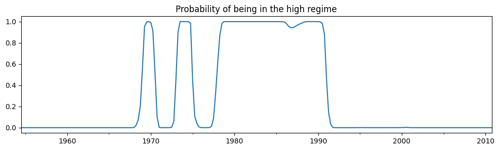
從摘要輸出中,第一個狀態(「低狀態」)中的平均聯邦基金利率估計為 \(3.7\),而在「高狀態」中則為 \(9.6\)。下面我們繪製處於高狀態的平滑機率。該模型表明 1980 年代是聯邦基金利率較高的時期。
[4]:
res_fedfunds.smoothed_marginal_probabilities[1].plot(
    title="Probability of being in the high regime", figsize=(12, 3)
)
[4]:
<Axes: title={'center': 'Probability of being in the high regime'}>
從估計的轉換矩陣中,我們可以計算出低狀態與高狀態的預期持續時間。
[5]:
print(res_fedfunds.expected_durations)
[55.85400626 19.85506546]
低狀態預計會持續約十四年,而高狀態預計只會持續約五年。
具有轉換截距和滯後因變數的聯邦基金利率
第二個範例擴充了之前的模型,以包括聯邦基金利率的滯後值。
其中 \(S_t \in \{0, 1\}\),且狀態轉換如下:
我們將透過最大似然法估計此模型的參數:\(p_{00}, p_{10}, \mu_0, \mu_1, \beta_0, \beta_1, \sigma^2\)。
[6]:
# Fit the model
mod_fedfunds2 = sm.tsa.MarkovRegression(
    dta_fedfunds.iloc[1:], k_regimes=2, exog=dta_fedfunds.iloc[:-1]
)
res_fedfunds2 = mod_fedfunds2.fit()
[7]:
res_fedfunds2.summary()
[7]:
| 因變數 | y | 觀測數量 | 225 |
|---|---|---|---|
| 模型 | MarkovRegression | 對數概度 | -264.711 |
| 日期 | 週四, 2024年10月03日 | AIC | 543.421 |
| 時間 | 15:45:38 | BIC | 567.334 |
| 樣本 | 10-01-1954 | HQIC | 553.073 |
| - 10-01-2010 | |||
| 共變異數類型 | 近似 |
| 係數 | 標準誤差 | z | P>|z| | [0.025 | 0.975] | |
|---|---|---|---|---|---|---|
| 常數 | 0.7245 | 0.289 | 2.510 | 0.012 | 0.159 | 1.290 |
| x1 | 0.7631 | 0.034 | 22.629 | 0.000 | 0.697 | 0.829 |
| 係數 | 標準誤差 | z | P>|z| | [0.025 | 0.975] | |
|---|---|---|---|---|---|---|
| 常數 | -0.0989 | 0.118 | -0.835 | 0.404 | -0.331 | 0.133 |
| x1 | 1.0612 | 0.019 | 57.351 | 0.000 | 1.025 | 1.097 |
| 係數 | 標準誤差 | z | P>|z| | [0.025 | 0.975] | |
|---|---|---|---|---|---|---|
| sigma2 | 0.4783 | 0.050 | 9.642 | 0.000 | 0.381 | 0.576 |
| 係數 | 標準誤差 | z | P>|z| | [0.025 | 0.975] | |
|---|---|---|---|---|---|---|
| p[0->0] | 0.6378 | 0.120 | 5.304 | 0.000 | 0.402 | 0.874 |
| p[1->0] | 0.1306 | 0.050 | 2.634 | 0.008 | 0.033 | 0.228 |
警告
[1] 共變異數矩陣是使用數值(複步)微分計算的。
從摘要輸出中,有幾件事值得注意:
資訊準則大幅下降,表明此模型比之前的模型更適合。
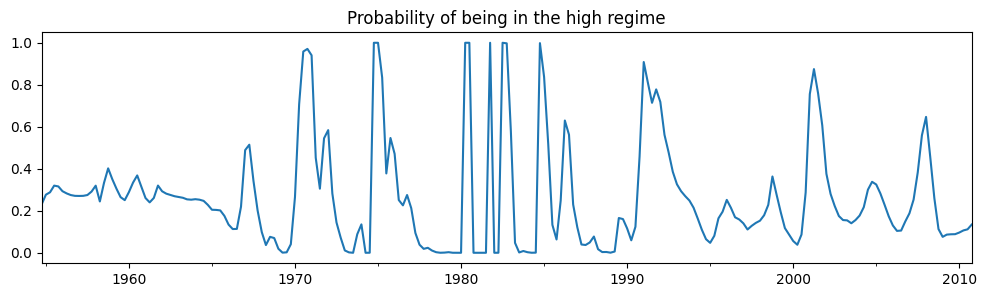
就截距而言,狀態的解釋已切換。現在,第一個狀態具有較高的截距,而第二個狀態具有較低的截距。
檢查高狀態的平滑機率,我們現在看到更多的變異性。
[8]:
res_fedfunds2.smoothed_marginal_probabilities[0].plot(
    title="Probability of being in the high regime", figsize=(12, 3)
)
[8]:
<Axes: title={'center': 'Probability of being in the high regime'}>
最後,每個狀態的預期持續時間都大幅減少。
[9]:
print(res_fedfunds2.expected_durations)
[2.76105188 7.65529154]
具有 2 個或 3 個狀態的泰勒法則
我們現在加入兩個額外的外生變數 - 產出缺口衡量指標和通貨膨脹衡量指標 - 以估計具有 2 個和 3 個狀態的轉換泰勒型法則,以查看哪個更適合數據。
由於這些模型通常難以估計,對於三狀態模型,我們採用了對起始參數的搜尋,以改善結果,並指定了 20 次隨機搜尋重複。
[10]:
# Get the additional data
from statsmodels.tsa.regime_switching.tests.test_markov_regression import ogap, inf

dta_ogap = pd.Series(ogap, index=pd.date_range("1954-07-01", "2010-10-01", freq="QS"))
dta_inf = pd.Series(inf, index=pd.date_range("1954-07-01", "2010-10-01", freq="QS"))

exog = pd.concat((dta_fedfunds.shift(), dta_ogap, dta_inf), axis=1).iloc[4:]

# Fit the 2-regime model
mod_fedfunds3 = sm.tsa.MarkovRegression(dta_fedfunds.iloc[4:], k_regimes=2, exog=exog)
res_fedfunds3 = mod_fedfunds3.fit()

# Fit the 3-regime model
np.random.seed(12345)
mod_fedfunds4 = sm.tsa.MarkovRegression(dta_fedfunds.iloc[4:], k_regimes=3, exog=exog)
res_fedfunds4 = mod_fedfunds4.fit(search_reps=20)
[11]:
res_fedfunds3.summary()
[11]:
| 因變數 | y | 觀測數量 | 222 |
|---|---|---|---|
| 模型 | MarkovRegression | 對數概度 | -229.256 |
| 日期 | 週四, 2024年10月03日 | AIC | 480.512 |
| 時間 | 15:45:42 | BIC | 517.942 |
| 樣本 | 07-01-1955 | HQIC | 495.624 |
| - 10-01-2010 | |||
| 共變異數類型 | 近似 |
| 係數 | 標準誤差 | z | P>|z| | [0.025 | 0.975] | |
|---|---|---|---|---|---|---|
| 常數 | 0.6555 | 0.137 | 4.771 | 0.000 | 0.386 | 0.925 |
| x1 | 0.8314 | 0.033 | 24.951 | 0.000 | 0.766 | 0.897 |
| x2 | 0.1355 | 0.029 | 4.609 | 0.000 | 0.078 | 0.193 |
| x3 | -0.0274 | 0.041 | -0.671 | 0.502 | -0.107 | 0.053 |
| 係數 | 標準誤差 | z | P>|z| | [0.025 | 0.975] | |
|---|---|---|---|---|---|---|
| 常數 | -0.0945 | 0.128 | -0.739 | 0.460 | -0.345 | 0.156 |
| x1 | 0.9293 | 0.027 | 34.309 | 0.000 | 0.876 | 0.982 |
| x2 | 0.0343 | 0.024 | 1.429 | 0.153 | -0.013 | 0.081 |
| x3 | 0.2125 | 0.030 | 7.147 | 0.000 | 0.154 | 0.271 |
| 係數 | 標準誤差 | z | P>|z| | [0.025 | 0.975] | |
|---|---|---|---|---|---|---|
| sigma2 | 0.3323 | 0.035 | 9.526 | 0.000 | 0.264 | 0.401 |
| 係數 | 標準誤差 | z | P>|z| | [0.025 | 0.975] | |
|---|---|---|---|---|---|---|
| p[0->0] | 0.7279 | 0.093 | 7.828 | 0.000 | 0.546 | 0.910 |
| p[1->0] | 0.2115 | 0.064 | 3.298 | 0.001 | 0.086 | 0.337 |
警告
[1] 共變異數矩陣是使用數值(複步)微分計算的。
[12]:
res_fedfunds4.summary()
[12]:
| 因變數 | y | 觀測數量 | 222 |
|---|---|---|---|
| 模型 | MarkovRegression | 對數概度 | -180.806 |
| 日期 | 週四, 2024年10月03日 | AIC | 399.611 |
| 時間 | 15:45:42 | BIC | 464.262 |
| 樣本 | 07-01-1955 | HQIC | 425.713 |
| - 10-01-2010 | |||
| 共變異數類型 | 近似 |
| 係數 | 標準誤差 | z | P>|z| | [0.025 | 0.975] | |
|---|---|---|---|---|---|---|
| 常數 | -1.0250 | 0.290 | -3.531 | 0.000 | -1.594 | -0.456 |
| x1 | 0.3277 | 0.086 | 3.812 | 0.000 | 0.159 | 0.496 |
| x2 | 0.2036 | 0.049 | 4.152 | 0.000 | 0.107 | 0.300 |
| x3 | 1.1381 | 0.081 | 13.977 | 0.000 | 0.978 | 1.298 |
| 係數 | 標準誤差 | z | P>|z| | [0.025 | 0.975] | |
|---|---|---|---|---|---|---|
| 常數 | -0.0259 | 0.087 | -0.298 | 0.765 | -0.196 | 0.144 |
| x1 | 0.9737 | 0.019 | 50.265 | 0.000 | 0.936 | 1.012 |
| x2 | 0.0341 | 0.017 | 2.030 | 0.042 | 0.001 | 0.067 |
| x3 | 0.1215 | 0.022 | 5.606 | 0.000 | 0.079 | 0.164 |
| 係數 | 標準誤差 | z | P>|z| | [0.025 | 0.975] | |
|---|---|---|---|---|---|---|
| 常數 | 0.7346 | 0.130 | 5.632 | 0.000 | 0.479 | 0.990 |
| x1 | 0.8436 | 0.024 | 35.198 | 0.000 | 0.797 | 0.891 |
| x2 | 0.1633 | 0.025 | 6.515 | 0.000 | 0.114 | 0.212 |
| x3 | -0.0499 | 0.027 | -1.835 | 0.067 | -0.103 | 0.003 |
| 係數 | 標準誤差 | z | P>|z| | [0.025 | 0.975] | |
|---|---|---|---|---|---|---|
| sigma2 | 0.1660 | 0.018 | 9.240 | 0.000 | 0.131 | 0.201 |
| 係數 | 標準誤差 | z | P>|z| | [0.025 | 0.975] | |
|---|---|---|---|---|---|---|
| p[0->0] | 0.7214 | 0.117 | 6.177 | 0.000 | 0.493 | 0.950 |
| p[1->0] | 4.001e-08 | nan | nan | nan | nan | nan |
| p[2->0] | 0.0783 | 0.038 | 2.079 | 0.038 | 0.004 | 0.152 |
| p[0->1] | 0.1044 | 0.095 | 1.103 | 0.270 | -0.081 | 0.290 |
| p[1->1] | 0.8259 | 0.054 | 15.208 | 0.000 | 0.719 | 0.932 |
| p[2->1] | 0.2288 | 0.073 | 3.150 | 0.002 | 0.086 | 0.371 |
警告
[1] 共變異數矩陣是使用數值(複步)微分計算的。
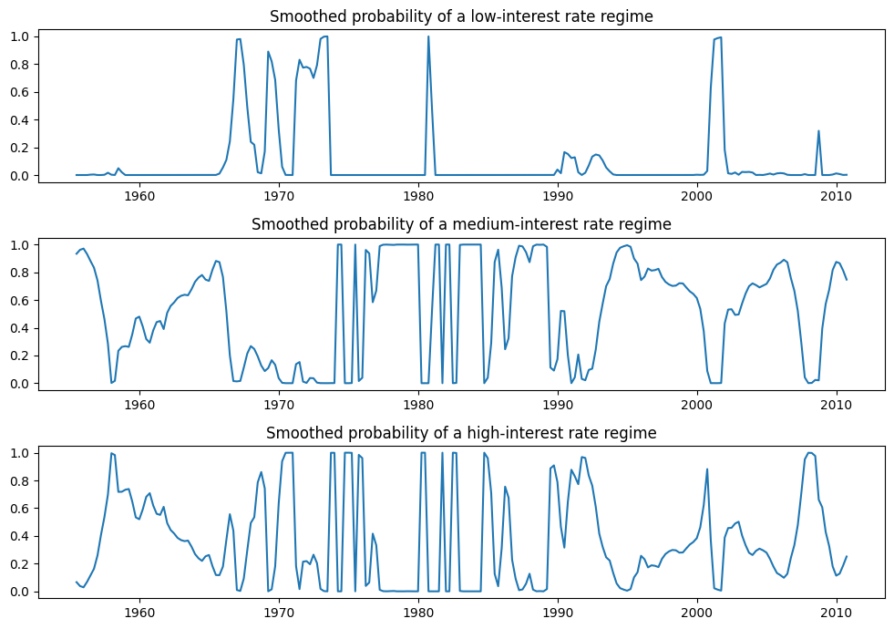
由於資訊準則較低,我們可能更喜歡三狀態模型,並將其解釋為低、中和高利率狀態。每個狀態的平滑機率繪製在下面。
[13]:
fig, axes = plt.subplots(3, figsize=(10, 7))

ax = axes[0]
ax.plot(res_fedfunds4.smoothed_marginal_probabilities[0])
ax.set(title="Smoothed probability of a low-interest rate regime")

ax = axes[1]
ax.plot(res_fedfunds4.smoothed_marginal_probabilities[1])
ax.set(title="Smoothed probability of a medium-interest rate regime")

ax = axes[2]
ax.plot(res_fedfunds4.smoothed_marginal_probabilities[2])
ax.set(title="Smoothed probability of a high-interest rate regime")

fig.tight_layout()
轉換變異數
我們也可以容納轉換變異數。特別是,我們考慮模型
我們使用最大似然法來估計此模型的參數:\(p_{00}, p_{10}, \mu_0, \mu_1, \beta_0, \beta_1, \sigma_0^2, \sigma_1^2\)。
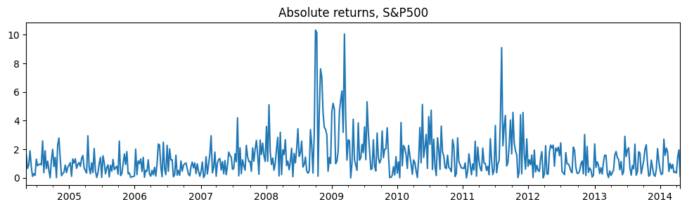
該應用是關於股票的絕對回報,數據可在 https://www.stata-press.com/data/r14/snp500 找到。
[14]:
# Get the federal funds rate data
from statsmodels.tsa.regime_switching.tests.test_markov_regression import areturns

dta_areturns = pd.Series(
    areturns, index=pd.date_range("2004-05-04", "2014-5-03", freq="W")
)

# Plot the data
dta_areturns.plot(title="Absolute returns, S&P500", figsize=(12, 3))

# Fit the model
mod_areturns = sm.tsa.MarkovRegression(
    dta_areturns.iloc[1:],
    k_regimes=2,
    exog=dta_areturns.iloc[:-1],
    switching_variance=True,
)
res_areturns = mod_areturns.fit()
[15]:
res_areturns.summary()
[15]:
| 因變數 | y | 觀測數量 | 520 |
|---|---|---|---|
| 模型 | MarkovRegression | 對數概度 | -745.798 |
| 日期 | 週四, 2024年10月03日 | AIC | 1507.595 |
| 時間 | 15:45:44 | BIC | 1541.626 |
| 樣本 | 05-16-2004 | HQIC | 1520.926 |
| - 04-27-2014 | |||
| 共變異數類型 | 近似 |
| 係數 | 標準誤差 | z | P>|z| | [0.025 | 0.975] | |
|---|---|---|---|---|---|---|
| 常數 | 0.7641 | 0.078 | 9.761 | 0.000 | 0.611 | 0.918 |
| x1 | 0.0791 | 0.030 | 2.620 | 0.009 | 0.020 | 0.138 |
| sigma2 | 0.3476 | 0.061 | 5.694 | 0.000 | 0.228 | 0.467 |
| 係數 | 標準誤差 | z | P>|z| | [0.025 | 0.975] | |
|---|---|---|---|---|---|---|
| 常數 | 1.9728 | 0.278 | 7.086 | 0.000 | 1.427 | 2.518 |
| x1 | 0.5280 | 0.086 | 6.155 | 0.000 | 0.360 | 0.696 |
| sigma2 | 2.5771 | 0.405 | 6.357 | 0.000 | 1.783 | 3.372 |
| 係數 | 標準誤差 | z | P>|z| | [0.025 | 0.975] | |
|---|---|---|---|---|---|---|
| p[0->0] | 0.7531 | 0.063 | 11.871 | 0.000 | 0.629 | 0.877 |
| p[1->0] | 0.6825 | 0.066 | 10.301 | 0.000 | 0.553 | 0.812 |
警告
[1] 共變異數矩陣是使用數值(複步)微分計算的。
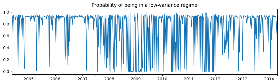
第一個狀態是低變異數狀態,第二個狀態是高變異數狀態。下面我們繪製處於低變異數狀態的機率。在 2008 年至 2012 年之間,似乎沒有明確的跡象表明有一個狀態在引導經濟。
[16]:
res_areturns.smoothed_marginal_probabilities[0].plot(
    title="Probability of being in a low-variance regime", figsize=(12, 3)
)
[16]:
<Axes: title={'center': 'Probability of being in a low-variance regime'}>