馬可夫轉換自迴歸模型
此筆記本提供在 statsmodels 中使用馬可夫轉換模型來複製 Kim 和 Nelson (1999) 中提出的一些結果的範例。它應用 Hamilton (1989) 的濾波器和 Kim (1994) 的平滑器。
這是針對 E-views 8 中的馬可夫轉換模型進行測試,可在http://www.eviews.com/EViews8/ev8ecswitch_n.html#MarkovAR找到,或是在 Stata 14 中的馬可夫轉換模型可在 http://www.stata.com/manuals14/tsmswitch.pdf找到。
[1]:
%matplotlib inline

from datetime import datetime
from io import BytesIO

import matplotlib.pyplot as plt
import numpy as np
import pandas as pd
import requests
import statsmodels.api as sm

# NBER recessions
from pandas_datareader.data import DataReader

usrec = DataReader(
    "USREC", "fred", start=datetime(1947, 1, 1), end=datetime(2013, 4, 1)
)
Hamilton (1989) GNP 轉換模型
這複製了 Hamilton (1989) 介紹馬可夫轉換模型的開創性論文。該模型是一個 4 階的自迴歸模型,其中過程的平均值在兩個狀態之間切換。它可以寫成
每個期間,狀態根據以下轉換機率矩陣轉換
其中 \(p_{ij}\) 是從狀態 \(i\) 轉換到狀態 \(j\) 的機率。
模型類別是 statsmodels 時間序列部分的 MarkovAutoregression。為了建立模型,我們必須指定狀態的數量,使用 k_regimes=2,以及自迴歸的階數,使用 order=4。預設模型也包含轉換自迴歸係數,因此在這裡我們也需要指定 switching_ar=False 以避免這種情況。
建立之後,通過最大概似估計來 fit 模型。在底層,使用期望最大化 (EM) 演算法的多個步驟來找到好的起始參數,並應用擬牛頓 (BFGS) 演算法來快速找到最大值。
[2]:
import requests
import shutil
def download_file(url):
local_filename = url.split('/')[-1]
with requests.get(url, stream=True) as r:
with open(local_filename, 'wb') as f:
shutil.copyfileobj(r.raw, f)
return local_filename
filename = download_file("https://www.stata-press.com/data/r14/rgnp.dta")
# Get the RGNP data to replicate Hamilton
dta = pd.read_stata(filename).iloc[1:]
dta.index = pd.DatetimeIndex(dta.date, freq="QS")
dta_hamilton = dta.rgnp
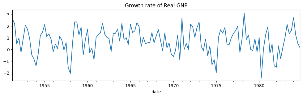
# Plot the data
dta_hamilton.plot(title="Growth rate of Real GNP", figsize=(12, 3))
# Fit the model
mod_hamilton = sm.tsa.MarkovAutoregression(
dta_hamilton, k_regimes=2, order=4, switching_ar=False
)
res_hamilton = mod_hamilton.fit()
[3]:
res_hamilton.summary()
[3]:
| 應變數 | rgnp | 觀測值數量 | 131 |
|---|---|---|---|
| 模型 | MarkovAutoregression | 對數概似值 | -181.263 |
| 日期 | 週四, 2024年10月03日 | AIC | 380.527 |
| 時間 | 15:44:58 | BIC | 406.404 |
| 樣本 | 04-01-1951 | HQIC | 391.042 |
| - 10-01-1984 | |||
| 共變異數類型 | approx |
| 係數 | 標準誤差 | z | P>|z| | [0.025 | 0.975] | |
|---|---|---|---|---|---|---|
| 常數 | -0.3588 | 0.265 | -1.356 | 0.175 | -0.877 | 0.160 |
| 係數 | 標準誤差 | z | P>|z| | [0.025 | 0.975] | |
|---|---|---|---|---|---|---|
| 常數 | 1.1635 | 0.075 | 15.614 | 0.000 | 1.017 | 1.310 |
| 係數 | 標準誤差 | z | P>|z| | [0.025 | 0.975] | |
|---|---|---|---|---|---|---|
| sigma2 | 0.5914 | 0.103 | 5.761 | 0.000 | 0.390 | 0.793 |
| ar.L1 | 0.0135 | 0.120 | 0.112 | 0.911 | -0.222 | 0.249 |
| ar.L2 | -0.0575 | 0.138 | -0.418 | 0.676 | -0.327 | 0.212 |
| ar.L3 | -0.2470 | 0.107 | -2.310 | 0.021 | -0.457 | -0.037 |
| ar.L4 | -0.2129 | 0.111 | -1.926 | 0.054 | -0.430 | 0.004 |
| 係數 | 標準誤差 | z | P>|z| | [0.025 | 0.975] | |
|---|---|---|---|---|---|---|
| p[0->0] | 0.7547 | 0.097 | 7.819 | 0.000 | 0.565 | 0.944 |
| p[1->0] | 0.0959 | 0.038 | 2.542 | 0.011 | 0.022 | 0.170 |
警告
[1] 共變異數矩陣是使用數值 (複數步) 微分計算的。
我們繪製了衰退的濾波和平滑機率。濾波指的是根據時間 \(t\)(但不包括時間 \(t+1, ..., T\))之前的數據對時間 \(t\) 的機率的估計。平滑指的是使用樣本中的所有數據對時間 \(t\) 的機率的估計。
為了參考,陰影期間代表 NBER 衰退期。
[4]:
fig, axes = plt.subplots(2, figsize=(7, 7))
ax = axes[0]
ax.plot(res_hamilton.filtered_marginal_probabilities[0])
ax.fill_between(usrec.index, 0, 1, where=usrec["USREC"].values, color="k", alpha=0.1)
ax.set_xlim(dta_hamilton.index[4], dta_hamilton.index[-1])
ax.set(title="Filtered probability of recession")

ax = axes[1]
ax.plot(res_hamilton.smoothed_marginal_probabilities[0])
ax.fill_between(usrec.index, 0, 1, where=usrec["USREC"].values, color="k", alpha=0.1)
ax.set_xlim(dta_hamilton.index[4], dta_hamilton.index[-1])
ax.set(title="Smoothed probability of recession")

fig.tight_layout()
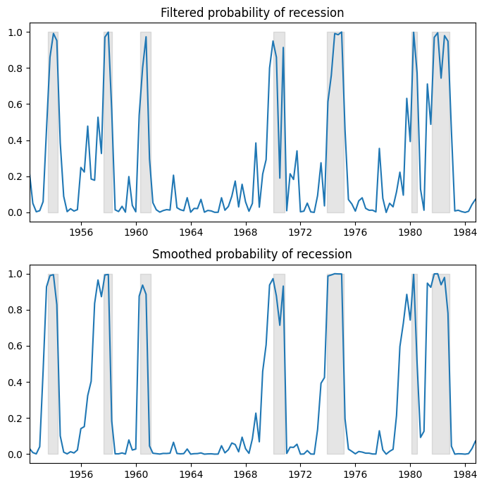
從估計的轉換矩陣中,我們可以計算出預期的衰退持續時間與擴張持續時間。
[5]:
print(res_hamilton.expected_durations)
[ 4.07604744 10.42589389]
在這種情況下,預計衰退將持續約一年(4 個季度),而擴張將持續約兩年半。
Kim, Nelson 和 Startz (1998) 三狀態變異數轉換
此模型演示了使用狀態異方差 (變異數轉換) 而無均值效應的估計。資料集可以在 http://econ.korea.ac.kr/~cjkim/MARKOV/data/ew_excs.prn 找到。
相關模型為
由於沒有自迴歸分量,因此可以使用 MarkovRegression 類別來擬合此模型。由於沒有均值效應,我們指定 trend='n'。假設有三個狀態用於轉換變異數,因此我們指定 k_regimes=3 和 switching_variance=True(預設情況下,假定變異數在各個狀態中是相同的)。
[6]:
# Get the dataset
ew_excs = requests.get("http://econ.korea.ac.kr/~cjkim/MARKOV/data/ew_excs.prn").content
raw = pd.read_table(BytesIO(ew_excs), header=None, skipfooter=1, engine="python")
raw.index = pd.date_range("1926-01-01", "1995-12-01", freq="MS")
dta_kns = raw.loc[:"1986"] - raw.loc[:"1986"].mean()
# Plot the dataset
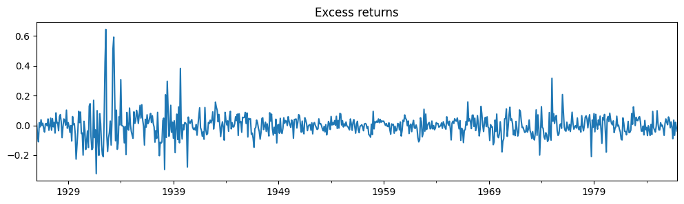
dta_kns[0].plot(title="Excess returns", figsize=(12, 3))
# Fit the model
mod_kns = sm.tsa.MarkovRegression(
dta_kns, k_regimes=3, trend="n", switching_variance=True
)
res_kns = mod_kns.fit()
[7]:
res_kns.summary()
[7]:
| 應變數 | 0 | 觀測值數量 | 732 |
|---|---|---|---|
| 模型 | MarkovRegression | 對數概似值 | 1001.895 |
| 日期 | 週四, 2024年10月03日 | AIC | -1985.790 |
| 時間 | 15:45:03 | BIC | -1944.428 |
| 樣本 | 01-01-1926 | HQIC | -1969.834 |
| - 12-01-1986 | |||
| 共變異數類型 | approx |
| 係數 | 標準誤差 | z | P>|z| | [0.025 | 0.975] | |
|---|---|---|---|---|---|---|
| sigma2 | 0.0012 | 0.000 | 7.136 | 0.000 | 0.001 | 0.002 |
| 係數 | 標準誤差 | z | P>|z| | [0.025 | 0.975] | |
|---|---|---|---|---|---|---|
| sigma2 | 0.0040 | 0.000 | 8.489 | 0.000 | 0.003 | 0.005 |
| 係數 | 標準誤差 | z | P>|z| | [0.025 | 0.975] | |
|---|---|---|---|---|---|---|
| sigma2 | 0.0311 | 0.006 | 5.461 | 0.000 | 0.020 | 0.042 |
| 係數 | 標準誤差 | z | P>|z| | [0.025 | 0.975] | |
|---|---|---|---|---|---|---|
| p[0->0] | 0.9747 | 0.000 | 7857.416 | 0.000 | 0.974 | 0.975 |
| p[1->0] | 0.0195 | 0.010 | 1.949 | 0.051 | -0.000 | 0.039 |
| p[2->0] | 2.354e-08 | nan | nan | nan | nan | nan |
| p[0->1] | 0.0253 | 3.97e-05 | 637.835 | 0.000 | 0.025 | 0.025 |
| p[1->1] | 0.9688 | 0.013 | 75.528 | 0.000 | 0.944 | 0.994 |
| p[2->1] | 0.0493 | 0.032 | 1.551 | 0.121 | -0.013 | 0.112 |
警告
[1] 共變異數矩陣是使用數值 (複數步) 微分計算的。
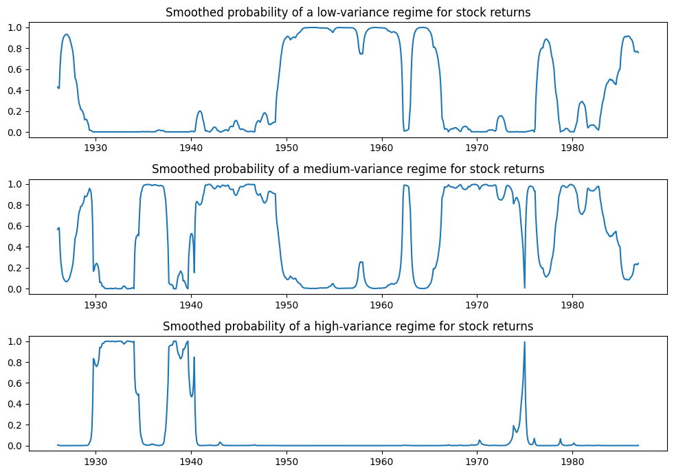
下面我們繪製了處於每個狀態的機率;僅在少數幾個時期,才可能出現高變異數狀態。
[8]:
fig, axes = plt.subplots(3, figsize=(10, 7))

ax = axes[0]
ax.plot(res_kns.smoothed_marginal_probabilities[0])
ax.set(title="Smoothed probability of a low-variance regime for stock returns")

ax = axes[1]
ax.plot(res_kns.smoothed_marginal_probabilities[1])
ax.set(title="Smoothed probability of a medium-variance regime for stock returns")

ax = axes[2]
ax.plot(res_kns.smoothed_marginal_probabilities[2])
ax.set(title="Smoothed probability of a high-variance regime for stock returns")

fig.tight_layout()
Filardo (1994) 時間變動的轉換機率
此模型演示了具有時間變動轉換機率的估計。資料集可以在 http://econ.korea.ac.kr/~cjkim/MARKOV/data/filardo.prn 找到。
在上述模型中,我們假設轉換機率在時間上是恆定的。這裡,我們允許機率隨經濟狀況的變化而變化。否則,該模型與 Hamilton (1989) 的馬可夫自迴歸相同。
每個期間,狀態現在根據以下時間變動的轉換機率矩陣轉換
其中 \(p_{ij,t}\) 是在期間 \(t\) 從狀態 \(i\) 轉換到狀態 \(j\) 的機率,並定義為
不是估計轉換機率作為最大概似的一部分,而是估計迴歸係數 \(\beta_{ij}\)。這些係數將轉換機率與預先確定或外生的迴歸變數 \(x_{t-1}\) 的向量相關聯。
[9]:
# Get the dataset
filardo = requests.get("http://econ.korea.ac.kr/~cjkim/MARKOV/data/filardo.prn").content
dta_filardo = pd.read_table(
BytesIO(filardo), sep=" +", header=None, skipfooter=1, engine="python"
)
dta_filardo.columns = ["month", "ip", "leading"]
dta_filardo.index = pd.date_range("1948-01-01", "1991-04-01", freq="MS")
dta_filardo["dlip"] = np.log(dta_filardo["ip"]).diff() * 100
# Deflated pre-1960 observations by ratio of std. devs.
# See hmt_tvp.opt or Filardo (1994) p. 302
std_ratio = (
dta_filardo["dlip"]["1960-01-01":].std() / dta_filardo["dlip"][:"1959-12-01"].std()
)
dta_filardo.loc[:"1959-12-01", "dlip"] = dta_filardo["dlip"][:"1959-12-01"] * std_ratio
dta_filardo["dlleading"] = np.log(dta_filardo["leading"]).diff() * 100
dta_filardo["dmdlleading"] = dta_filardo["dlleading"] - dta_filardo["dlleading"].mean()
# Plot the data
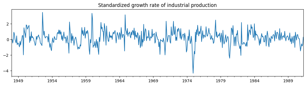
dta_filardo["dlip"].plot(
title="Standardized growth rate of industrial production", figsize=(13, 3)
)
plt.figure()
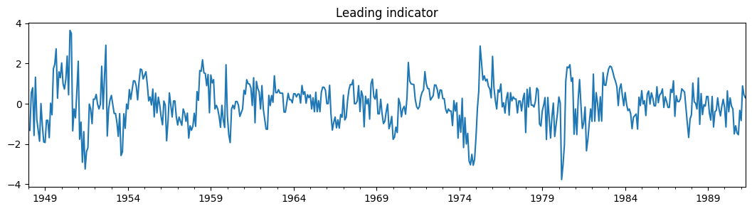
dta_filardo["dmdlleading"].plot(title="Leading indicator", figsize=(13, 3))
[9]:
<Axes: title={'center': 'Leading indicator'}>
時間變動的轉換機率由 exog_tvtp 參數指定。
這裡我們演示了模型擬合的另一個功能 - 使用隨機搜尋來尋找 MLE 起始參數。由於馬可夫轉換模型通常以概似函數的許多局部最大值為特徵,因此執行初始優化步驟可能有助於找到最佳參數。
下面,我們指定檢視起始參數向量的 20 個隨機擾動,並將最佳的一個用作實際的起始參數。由於搜尋的隨機性,我們事先對隨機數產生器進行播種,以便可以複製結果。
[10]:
mod_filardo = sm.tsa.MarkovAutoregression(
    dta_filardo.iloc[2:]["dlip"],
    k_regimes=2,
    order=4,
    switching_ar=False,
    exog_tvtp=sm.add_constant(dta_filardo.iloc[1:-1]["dmdlleading"]),
)

np.random.seed(12345)
res_filardo = mod_filardo.fit(search_reps=20)
[11]:
res_filardo.summary()
[11]:
| 應變數 | dlip | 觀測值數量 | 514 |
|---|---|---|---|
| 模型 | MarkovAutoregression | 對數概似值 | -586.572 |
| 日期 | 週四, 2024年10月03日 | AIC | 1195.144 |
| 時間 | 15:45:14 | BIC | 1241.808 |
| 樣本 | 03-01-1948 | HQIC | 1213.433 |
| - 04-01-1991 | |||
| 共變異數類型 | approx |
| 係數 | 標準誤差 | z | P>|z| | [0.025 | 0.975] | |
|---|---|---|---|---|---|---|
| 常數 | -0.8659 | 0.153 | -5.658 | 0.000 | -1.166 | -0.566 |
| 係數 | 標準誤差 | z | P>|z| | [0.025 | 0.975] | |
|---|---|---|---|---|---|---|
| 常數 | 0.5173 | 0.077 | 6.706 | 0.000 | 0.366 | 0.668 |
| 係數 | 標準誤差 | z | P>|z| | [0.025 | 0.975] | |
|---|---|---|---|---|---|---|
| sigma2 | 0.4844 | 0.037 | 13.172 | 0.000 | 0.412 | 0.556 |
| ar.L1 | 0.1895 | 0.050 | 3.761 | 0.000 | 0.091 | 0.288 |
| ar.L2 | 0.0793 | 0.051 | 1.552 | 0.121 | -0.021 | 0.180 |
| ar.L3 | 0.1109 | 0.052 | 2.136 | 0.033 | 0.009 | 0.213 |
| ar.L4 | 0.1223 | 0.051 | 2.418 | 0.016 | 0.023 | 0.221 |
| 係數 | 標準誤差 | z | P>|z| | [0.025 | 0.975] | |
|---|---|---|---|---|---|---|
| p[0->0].tvtp0 | 1.6494 | 0.446 | 3.702 | 0.000 | 0.776 | 2.523 |
| p[1->0].tvtp0 | -4.3595 | 0.747 | -5.833 | 0.000 | -5.824 | -2.895 |
| p[0->0].tvtp1 | -0.9945 | 0.566 | -1.758 | 0.079 | -2.103 | 0.114 |
| p[1->0].tvtp1 | -1.7702 | 0.508 | -3.484 | 0.000 | -2.766 | -0.775 |
警告
[1] 共變異數矩陣是使用數值 (複數步) 微分計算的。
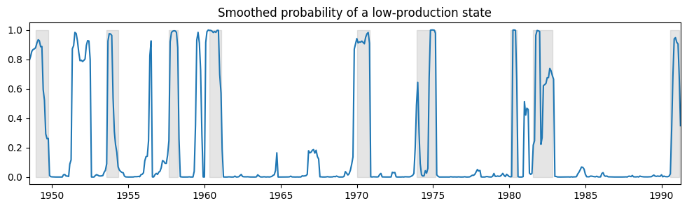
下面我們繪製了經濟在低產出狀態下運作的平滑機率,並再次包含 NBER 衰退期以進行比較。
[12]:
fig, ax = plt.subplots(figsize=(12, 3))

ax.plot(res_filardo.smoothed_marginal_probabilities[0])
ax.fill_between(usrec.index, 0, 1, where=usrec["USREC"].values, color="gray", alpha=0.2)
ax.set_xlim(dta_filardo.index[6], dta_filardo.index[-1])
ax.set(title="Smoothed probability of a low-production state")
[12]:
[Text(0.5, 1.0, 'Smoothed probability of a low-production state')]
使用時間變動的轉換機率,我們可以了解低產出狀態的預期持續時間如何隨時間變化
[13]:
res_filardo.expected_durations[0].plot(
    title="Expected duration of a low-production state", figsize=(12, 3)
)
[13]:
<Axes: title={'center': 'Expected duration of a low-production state'}>
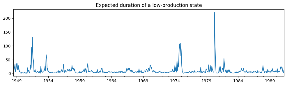
在衰退期間,低產出狀態的預期持續時間遠高於擴張期間。