失業率的趨勢與週期
在這裡,我們考慮三種分離經濟資料中趨勢和週期的方法。假設我們有一個時間序列 \(y_t\),基本想法是將其分解為以下兩個成分
\[y_t = \mu_t + \eta_t\]
其中 \(\mu_t\) 代表趨勢或水平,而 \(\eta_t\) 代表週期性成分。在這種情況下,我們考慮的是隨機趨勢,因此 \(\mu_t\) 是一個隨機變數,而不是時間的確定性函數。其中兩種方法屬於「未觀測成分」模型的範疇,第三種方法是廣受歡迎的霍德里克-普雷斯科特 (HP) 濾波器。與例如 Harvey 和 Jaeger (1993) 的研究一致,我們發現這些模型都產生相似的分解結果。
這個筆記本示範了如何應用這些模型來分離美國失業率的趨勢和週期。
[1]:
%matplotlib inline
[2]:
import numpy as np
import pandas as pd
import statsmodels.api as sm
import matplotlib.pyplot as plt
[3]:
from pandas_datareader.data import DataReader
endog = DataReader('UNRATE', 'fred', start='1954-01-01')
endog.index.freq = endog.index.inferred_freq
霍德里克-普雷斯科特 (HP) 濾波器
第一種方法是霍德里克-普雷斯科特濾波器,可以以非常直接的方法應用於資料序列。在這裡,我們指定參數 \(\lambda=129600\),因為失業率是按月觀測的。
[4]:
hp_cycle, hp_trend = sm.tsa.filters.hpfilter(endog, lamb=129600)
未觀測成分和 ARIMA 模型 (UC-ARIMA)
下一個方法是未觀測成分模型,其中趨勢被建模為隨機漫步,而週期則使用 ARIMA 模型建模 - 特別是,在這裡我們使用 AR(4) 模型。時間序列的過程可以寫成
\[\begin{split}\begin{align} y_t & = \mu_t + \eta_t \\ \mu_{t+1} & = \mu_t + \epsilon_{t+1} \\ \phi(L) \eta_t & = \nu_t \end{align}\end{split}\]
其中 \(\phi(L)\) 是 AR(4) 延遲多項式,而 \(\epsilon_t\) 和 \(\nu_t\) 是白雜訊。
[5]:
mod_ucarima = sm.tsa.UnobservedComponents(endog, 'rwalk', autoregressive=4)
# Here the powell method is used, since it achieves a
# higher loglikelihood than the default L-BFGS method
res_ucarima = mod_ucarima.fit(method='powell', disp=False)
print(res_ucarima.summary())
                        Unobserved Components Results
==============================================================================
Dep. Variable:                 UNRATE   No. Observations:                  848
Model:                    random walk   Log Likelihood                -463.716
                              + AR(4)   AIC                            939.431
Date:                Thu, 03 Oct 2024   BIC                            967.881
Time:                        15:46:35   HQIC                           950.331
Sample:                    01-01-1954
                         - 08-01-2024
Covariance Type:                  opg
================================================================================
                   coef    std err          z      P>|z|      [0.025      0.975]
--------------------------------------------------------------------------------
sigma2.level  5.487e-08      0.011   4.92e-06      1.000      -0.022       0.022
sigma2.ar        0.1746      0.015     11.697      0.000       0.145       0.204
ar.L1            1.0256      0.019     54.095      0.000       0.988       1.063
ar.L2           -0.1059      0.016     -6.600      0.000      -0.137      -0.074
ar.L3            0.0756      0.023      3.271      0.001       0.030       0.121
ar.L4           -0.0267      0.019     -1.421      0.155      -0.064       0.010
===================================================================================
Ljung-Box (L1) (Q):                   0.00   Jarque-Bera (JB):           6657871.78
Prob(Q):                              0.97   Prob(JB):                         0.00
Heteroskedasticity (H):               9.13   Skew:                            17.46
Prob(H) (two-sided):                  0.00   Kurtosis:                       435.94
===================================================================================

Warnings:
[1] Covariance matrix calculated using the outer product of gradients (complex-step).
具有隨機週期的未觀測成分 (UC)
最後一種方法也是未觀測成分模型,但其中週期是顯式建模的。
\[\begin{split}\begin{align} y_t & = \mu_t + \eta_t \\ \mu_{t+1} & = \mu_t + \epsilon_{t+1} \\ \eta_{t+1} & = \eta_t \cos \lambda_\eta + \eta_t^* \sin \lambda_\eta + \tilde \omega_t \qquad & \tilde \omega_t \sim N(0, \sigma_{\tilde \omega}^2) \\ \eta_{t+1}^* & = -\eta_t \sin \lambda_\eta + \eta_t^* \cos \lambda_\eta + \tilde \omega_t^* & \tilde \omega_t^* \sim N(0, \sigma_{\tilde \omega}^2) \end{align}\end{split}\]
[6]:
mod_uc = sm.tsa.UnobservedComponents(
    endog, 'rwalk',
    cycle=True, stochastic_cycle=True, damped_cycle=True,
)
# Here the powell method gets close to the optimum
res_uc = mod_uc.fit(method='powell', disp=False)
# but to get to the highest loglikelihood we do a
# second round using the L-BFGS method.
res_uc = mod_uc.fit(res_uc.params, disp=False)
print(res_uc.summary())
                            Unobserved Components Results
=====================================================================================
Dep. Variable:                        UNRATE   No. Observations:                  848
Model:                           random walk   Log Likelihood                -472.478
                   + damped stochastic cycle   AIC                            952.956
Date:                       Thu, 03 Oct 2024   BIC                            971.913
Time:                               15:46:37   HQIC                           960.219
Sample:                           01-01-1954
                                - 08-01-2024
Covariance Type:                         opg
===================================================================================
                      coef    std err          z      P>|z|      [0.025      0.975]
-----------------------------------------------------------------------------------
sigma2.level        0.0183      0.033      0.552      0.581      -0.047       0.083
sigma2.cycle        0.1539      0.032      4.740      0.000       0.090       0.217
frequency.cycle     0.0437      0.029      1.495      0.135      -0.014       0.101
damping.cycle       0.9562      0.019     51.074      0.000       0.919       0.993
===================================================================================
Ljung-Box (L1) (Q):                   1.53   Jarque-Bera (JB):           6560083.72
Prob(Q):                              0.22   Prob(JB):                         0.00
Heteroskedasticity (H):               9.47   Skew:                            17.32
Prob(H) (two-sided):                  0.00   Kurtosis:                       433.26
===================================================================================

Warnings:
[1] Covariance matrix calculated using the outer product of gradients (complex-step).
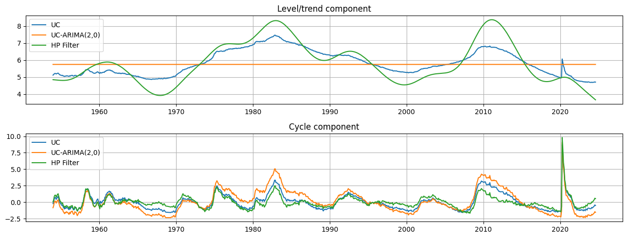
圖形比較
每個模型的輸出都是趨勢成分 \(\mu_t\) 和週期成分 \(\eta_t\) 的估計值。趨勢和週期的估計在質量上非常相似,儘管 HP 濾波器中的趨勢成分比未觀測成分模型中的趨勢成分更具變異性。這意味著失業率的變動相對而言,更多歸因於潛在趨勢的變化,而不是暫時性的週期性波動。
[7]:
fig, axes = plt.subplots(2, figsize=(13,5));
axes[0].set(title='Level/trend component')
axes[0].plot(endog.index, res_uc.level.smoothed, label='UC')
axes[0].plot(endog.index, res_ucarima.level.smoothed, label='UC-ARIMA(2,0)')
axes[0].plot(hp_trend, label='HP Filter')
axes[0].legend(loc='upper left')
axes[0].grid()

axes[1].set(title='Cycle component')
axes[1].plot(endog.index, res_uc.cycle.smoothed, label='UC')
axes[1].plot(endog.index, res_ucarima.autoregressive.smoothed, label='UC-ARIMA(2,0)')
axes[1].plot(hp_cycle, label='HP Filter')
axes[1].legend(loc='upper left')
axes[1].grid()

fig.tight_layout();
上次更新:2024 年 10 月 03 日