SARIMAX 和 ARIMA:常見問題 (FAQ)
此筆記本包含常見問題的解釋。
比較
SARIMAX、ARIMA和AutoReg中的趨勢和外生變數在
SARIMAX和ARIMA中重建殘差、擬合值和預測SARIMAX和ARIMA中的初始殘差
比較 SARIMAX、ARIMA 和 AutoReg 中的趨勢和外生變數
ARIMA 在形式上是具有 ARMA 誤差的 OLS。具有 ARMA 誤差的 OLS 中的基本 AR(1) 描述為
在大型樣本中,\(\hat{\delta}\stackrel{p}{\rightarrow} E[Y]\)。
SARIMAX 使用不同的表示法,因此當使用 SARIMAX 估計時,模型為
這與使用 OLS (AutoReg) 估計模型時使用的表示法相同。在大型樣本中,\(\hat{\phi}\stackrel{p}{\rightarrow} E[Y](1-\rho)\)。
在下一個儲存格中,我們模擬一個大型樣本並驗證這些關係在實務中是否成立。
[1]:
%matplotlib inline
[2]:
import numpy as np
import pandas as pd

rng = np.random.default_rng(20210819)
eta = rng.standard_normal(5200)
rho = 0.8
beta = 10
epsilon = eta.copy()
for i in range(1, eta.shape[0]):
    epsilon[i] = rho * epsilon[i - 1] + eta[i]
y = beta + epsilon
y = y[200:]
[3]:
from statsmodels.tsa.api import SARIMAX, AutoReg
from statsmodels.tsa.arima.model import ARIMA
在下一個儲存格中,指定並估計了這三個模型。包含 AR(0) 作為參考。使用所有三個估計器,AR(0) 是相同的。
[4]:
ar0_res = SARIMAX(y, order=(0, 0, 0), trend="c").fit()
sarimax_res = SARIMAX(y, order=(1, 0, 0), trend="c").fit()
arima_res = ARIMA(y, order=(1, 0, 0), trend="c").fit()
autoreg_res = AutoReg(y, 1, trend="c").fit()
 This problem is unconstrained.
 This problem is unconstrained.
RUNNING THE L-BFGS-B CODE

           * * *

Machine precision = 2.220D-16
 N =            2     M =           10

At X0         0 variables are exactly at the bounds

At iterate    0    f=  1.91760D+00    |proj g|=  3.68860D-06

           * * *

Tit   = total number of iterations
Tnf   = total number of function evaluations
Tnint = total number of segments explored during Cauchy searches
Skip  = number of BFGS updates skipped
Nact  = number of active bounds at final generalized Cauchy point
Projg = norm of the final projected gradient
F     = final function value

           * * *

   N    Tit     Tnf  Tnint  Skip  Nact     Projg        F
    2      0      1      0     0     0   3.689D-06   1.918D+00
  F =   1.9175996129577773

CONVERGENCE: NORM_OF_PROJECTED_GRADIENT_<=_PGTOL
RUNNING THE L-BFGS-B CODE

           * * *

Machine precision = 2.220D-16
 N =            3     M =           10

At X0         0 variables are exactly at the bounds

At iterate    0    f=  1.41373D+00    |proj g|=  9.51828D-04

           * * *

Tit   = total number of iterations
Tnf   = total number of function evaluations
Tnint = total number of segments explored during Cauchy searches
Skip  = number of BFGS updates skipped
Nact  = number of active bounds at final generalized Cauchy point
Projg = norm of the final projected gradient
F     = final function value

           * * *

   N    Tit     Tnf  Tnint  Skip  Nact     Projg        F
    3      2      5      1     0     0   4.516D-05   1.414D+00
  F =   1.4137311050015484

CONVERGENCE: REL_REDUCTION_OF_F_<=_FACTR*EPSMCH
下表包含模型中估計的參數、估計的 AR(1) 係數和長期平均值,長期平均值等於估計的參數 (AR(0) 或 ARIMA),或取決於截距與 1 減去 AR(1) 參數的比率。
[5]:
intercept = [
    ar0_res.params[0],
    sarimax_res.params[0],
    arima_res.params[0],
    autoreg_res.params[0],
]
rho_hat = [0] + [r.params[1] for r in (sarimax_res, arima_res, autoreg_res)]
long_run = [
    ar0_res.params[0],
    sarimax_res.params[0] / (1 - sarimax_res.params[1]),
    arima_res.params[0],
    autoreg_res.params[0] / (1 - autoreg_res.params[1]),
]
cols = ["AR(0)", "SARIMAX", "ARIMA", "AutoReg"]
pd.DataFrame(
    [intercept, rho_hat, long_run],
    columns=cols,
    index=["delta-or-phi", "rho", "long-run mean"],
)
[5]:
| AR(0) | SARIMAX | ARIMA | AutoReg | |
|---|---|---|---|---|
| delta-or-phi | 9.7745 | 1.985714 | 9.774498 | 1.985790 |
| rho | 0.0000 | 0.796846 | 0.796875 | 0.796882 |
| 長期平均值 | 9.7745 | 9.774424 | 9.774498 | 9.776537 |
SARIMAX 中趨勢和 exog 之間的差異
當 SARIMAX 包含 exog 變數時,exog 被視為 OLS 迴歸變數,因此估計的模型為
在下一個範例中,我們省略了趨勢,而是包含了一個 1 的欄位,這產生一個模型,在大型樣本中,它與沒有外生迴歸變數且 trend="c" 的情況等效。此處 const 的估計值與使用 ARIMA 估計的值相符。之所以會發生這種情況,是因為 SARIMAX 中的 exog 和 ARIMA 中的趨勢都被視為具有 ARMA 誤差的線性迴歸模型。
[6]:
sarimax_exog_res = SARIMAX(y, exog=np.ones_like(y), order=(1, 0, 0), trend="n").fit()
print(sarimax_exog_res.summary())
RUNNING THE L-BFGS-B CODE

           * * *

Machine precision = 2.220D-16
 N =            3     M =           10

At X0         0 variables are exactly at the bounds

At iterate    0    f=  1.41373D+00    |proj g|=  1.06920D-04

           * * *

Tit   = total number of iterations
Tnf   = total number of function evaluations
Tnint = total number of segments explored during Cauchy searches
Skip  = number of BFGS updates skipped
Nact  = number of active bounds at final generalized Cauchy point
Projg = norm of the final projected gradient
F     = final function value

           * * *

   N    Tit     Tnf  Tnint  Skip  Nact     Projg        F
    3      1      4      1     0     0   4.752D-05   1.414D+00
  F =   1.4137311099487531

CONVERGENCE: REL_REDUCTION_OF_F_<=_FACTR*EPSMCH
This problem is unconstrained.
                               SARIMAX Results
==============================================================================
Dep. Variable:                      y   No. Observations:                 5000
Model:               SARIMAX(1, 0, 0)   Log Likelihood               -7068.656
Date:                Thu, 03 Oct 2024   AIC                          14143.311
Time:                        15:45:04   BIC                          14162.863
Sample:                             0   HQIC                         14150.164
                               - 5000
Covariance Type:                  opg
==============================================================================
                 coef    std err          z      P>|z|      [0.025      0.975]
------------------------------------------------------------------------------
const          9.7745      0.069    141.177      0.000       9.639       9.910
ar.L1          0.7969      0.009     93.691      0.000       0.780       0.814
sigma2         0.9894      0.020     49.921      0.000       0.951       1.028
===================================================================================
Ljung-Box (L1) (Q):                   0.42   Jarque-Bera (JB):                 0.08
Prob(Q):                              0.51   Prob(JB):                         0.96
Heteroskedasticity (H):               0.97   Skew:                            -0.01
Prob(H) (two-sided):                  0.47   Kurtosis:                         2.99
===================================================================================

Warnings:
[1] Covariance matrix calculated using the outer product of gradients (complex-step).
在 SARIMAX 和 ARIMA 中使用 exog
雖然在這兩個模型中,exog 的處理方式相同,但截距仍然不同。在下面,我們將外生迴歸變數新增到 y,然後使用所有三種方法擬合模型。現在的資料產生過程為
[7]:
full_x = rng.standard_normal(eta.shape)
x = full_x[200:]
y += 3 * x
[8]:
sarimax_exog_res = SARIMAX(y, exog=x, order=(1, 0, 0), trend="c").fit()
arima_exog_res = ARIMA(y, exog=x, order=(1, 0, 0), trend="c").fit()
RUNNING THE L-BFGS-B CODE

           * * *

Machine precision = 2.220D-16
 N =            4     M =           10

At X0         0 variables are exactly at the bounds

At iterate    0    f=  1.42683D+00    |proj g|=  2.05943D-01
This problem is unconstrained.
At iterate    5    f=  1.41332D+00    |proj g|=  1.60874D-03

At iterate   10    f=  1.41329D+00    |proj g|=  3.11659D-05

           * * *

Tit   = total number of iterations
Tnf   = total number of function evaluations
Tnint = total number of segments explored during Cauchy searches
Skip  = number of BFGS updates skipped
Nact  = number of active bounds at final generalized Cauchy point
Projg = norm of the final projected gradient
F     = final function value

           * * *

   N    Tit     Tnf  Tnint  Skip  Nact     Projg        F
    4     11     15      1     0     0   1.796D-06   1.413D+00
  F =   1.4132928400115858

CONVERGENCE: NORM_OF_PROJECTED_GRADIENT_<=_PGTOL
檢查參數表,我們看到 x1 的參數估計值是相同的,而 intercept 的估計值由於這些估計器中趨勢處理方式的差異而繼續不同。
SARIMAX
[9]:
def print_params(s):
    from io import StringIO

    return pd.read_csv(StringIO(s.tables[1].as_csv()), index_col=0)


print_params(sarimax_exog_res.summary())
[9]:
| coef | std err | z | P>|z| | [0.025 | 0.975] | |
|---|---|---|---|---|---|---|
| intercept | 1.9849 | 0.085 | 23.484 | 0.0 | 1.819 | 2.151 |
| x1 | 3.0231 | 0.011 | 277.150 | 0.0 | 3.002 | 3.044 |
| ar.L1 | 0.7969 | 0.009 | 93.735 | 0.0 | 0.780 | 0.814 |
| sigma2 | 0.9886 | 0.020 | 49.941 | 0.0 | 0.950 | 1.027 |
ARIMA
[10]:
print_params(arima_exog_res.summary())
[10]:
| coef | std err | z | P>|z| | [0.025 | 0.975] | |
|---|---|---|---|---|---|---|
| const | 9.7741 | 0.069 | 141.201 | 0.0 | 9.638 | 9.910 |
| x1 | 3.0231 | 0.011 | 277.140 | 0.0 | 3.002 | 3.044 |
| ar.L1 | 0.7969 | 0.009 | 93.728 | 0.0 | 0.780 | 0.814 |
| sigma2 | 0.9886 | 0.020 | 49.941 | 0.0 | 0.950 | 1.027 |
AutoReg 中的 exog
當使用 AutoReg 使用 OLS 估計模型時,該模型與 SARIMAX 和 ARIMA 不同。具有外生變數的 AutoReg 規格為
此規格不等效於 SARIMAX 和 ARIMA 中估計的規格。此處的差異並非微不足道,在相同的時間序列上進行樸素估計會導致不同的參數值,即使在大型樣本中也是如此(以及極限)。估計此模型會變更 AR(1) 係數的參數估計值。
AutoReg
[11]:
autoreg_exog_res = AutoReg(y, 1, exog=x, trend="c").fit()
print_params(autoreg_exog_res.summary())
[11]:
| coef | std err | z | P>|z| | [0.025 | 0.975] | |
|---|---|---|---|---|---|---|
| const | 7.9714 | 0.064 | 124.525 | 0.0 | 7.846 | 8.097 |
| y.L1 | 0.1838 | 0.006 | 29.890 | 0.0 | 0.172 | 0.196 |
| x1 | 3.0311 | 0.021 | 142.513 | 0.0 | 2.989 | 3.073 |
關鍵差異可以透過使用滯後運算子表示法寫出模型來看出。
其中假設 \(|\phi|<1\)。此處我們看到 \(Y_t\) 取決於 \(X_t\) 和 \(\eta_t\) 的所有滯後值。這與 SARIMAX 和 ARIMA 估計的規格不同,可以看出是
在本規範中,\(Y_t\) 僅取決於 \(X_t\),而不取決於其他落後期數。
使用 AutoReg 的正確資料生成過程 (DGP)
模擬在 AutoReg 中估計的過程顯示,參數是從真實模型中恢復的。
[12]:
y = beta + eta
epsilon = eta.copy()
for i in range(1, eta.shape[0]):
    y[i] = beta * (1 - rho) + rho * y[i - 1] + 3 * full_x[i] + eta[i]
y = y[200:]
使用正確 DGP 的 AutoReg
[13]:
autoreg_alt_exog_res = AutoReg(y, 1, exog=x, trend="c").fit()
print_params(autoreg_alt_exog_res.summary())
[13]:
| coef | std err | z | P>|z| | [0.025 | 0.975] | |
|---|---|---|---|---|---|---|
| const | 1.9870 | 0.030 | 66.526 | 0.0 | 1.928 | 2.046 |
| y.L1 | 0.7968 | 0.003 | 300.382 | 0.0 | 0.792 | 0.802 |
| x1 | 3.0263 | 0.014 | 217.034 | 0.0 | 2.999 | 3.054 |
在 SARIMAX 和 ARIMA 中重建殘差、擬合值和預測值
在僅包含自迴歸項、趨勢和外生變數的模型中,一旦達到模型中的最大落後期數,就可以輕鬆地重建擬合值和預測值。在實務上,這意味著在 \((P+D)s+p+d\) 個期間之後。較早的預測和殘差較難重建,因為該模型會為 \(Y_t|Y_{t-1},Y_{t-2},...\) 建立最佳預測。當 \(Y\) 的落後期數小於自迴歸階數時,最佳預測的表達式與模型不同。例如,在預測第一個值 \(Y_1\) 時,沒有來自 \(Y\) 歷史的可用資訊,因此最佳預測是無條件平均值。在 AR(1) 的情況下,第二個預測將遵循模型,因此在使用 ARIMA 時,預測為
因為 ARIMA 將外生和趨勢項都視為具有 ARMA 誤差的迴歸。
這可以在接下來的單元格中看到。
[14]:
arima_res = ARIMA(y, order=(1, 0, 0), trend="c").fit()
print_params(arima_res.summary())
[14]:
| coef | std err | z | P>|z| | [0.025 | 0.975] | |
|---|---|---|---|---|---|---|
| const | 9.9346 | 0.222 | 44.667 | 0.0 | 9.499 | 10.371 |
| ar.L1 | 0.7957 | 0.009 | 92.515 | 0.0 | 0.779 | 0.813 |
| sigma2 | 10.3015 | 0.204 | 50.496 | 0.0 | 9.902 | 10.701 |
[15]:
arima_res.predict(0, 2)
[15]:
array([ 9.93458658, 10.91088035, 11.80415747])
[16]:
delta_hat, rho_hat = arima_res.params[:2]
delta_hat + rho_hat * (y[0] - delta_hat)
[16]:
np.float64(10.910880346250012)
SARIMAX 以不同的方式處理趨勢項,因此使用 SARIMAX 估計的模型產生的一步預測為
[17]:
sarima_res = SARIMAX(y, order=(1, 0, 0), trend="c").fit()
print_params(sarima_res.summary())
RUNNING THE L-BFGS-B CODE

           * * *

Machine precision = 2.220D-16
 N =            3     M =           10

At X0         0 variables are exactly at the bounds

At iterate    0    f=  2.58518D+00    |proj g|=  5.99456D-05

           * * *

Tit   = total number of iterations
Tnf   = total number of function evaluations
Tnint = total number of segments explored during Cauchy searches
Skip  = number of BFGS updates skipped
Nact  = number of active bounds at final generalized Cauchy point
Projg = norm of the final projected gradient
F     = final function value

           * * *

   N    Tit     Tnf  Tnint  Skip  Nact     Projg        F
    3      3      5      1     0     0   3.347D-05   2.585D+00
  F =   2.5851830060985752

CONVERGENCE: REL_REDUCTION_OF_F_<=_FACTR*EPSMCH
This problem is unconstrained.
[17]:
| coef | std err | z | P>|z| | [0.025 | 0.975] | |
|---|---|---|---|---|---|---|
| intercept | 2.0283 | 0.097 | 20.841 | 0.0 | 1.838 | 2.219 |
| ar.L1 | 0.7959 | 0.009 | 92.536 | 0.0 | 0.779 | 0.813 |
| sigma2 | 10.3007 | 0.204 | 50.500 | 0.0 | 9.901 | 10.700 |
[18]:
sarima_res.predict(0, 2)
[18]:
array([ 9.93588659, 10.91128867, 11.80469658])
[19]:
delta_hat, rho_hat = sarima_res.params[:2]
delta_hat + rho_hat * y[0]
[19]:
np.float64(10.911288670367867)
具有 MA 成分的預測
當模型包含 MA 成分時,預測會更加複雜,因為誤差永遠無法直接觀察到。預測仍然是 \(Y_t|Y_{t-1},Y_{t-2},...\),當 MA 成分可逆時,最佳預測可以表示為 \(t\)-lag AR 過程。當 \(t\) 很大時,這應該非常接近於假設誤差可觀察時的預測。對於較短的落後,這可能會明顯不同。
在下一個單元格中,我們模擬一個 MA(1) 過程,並擬合一個 MA 模型。
[20]:
rho = 0.8
beta = 10
epsilon = eta.copy()
for i in range(1, eta.shape[0]):
    epsilon[i] = rho * eta[i - 1] + eta[i]
y = beta + epsilon
y = y[200:]

ma_res = ARIMA(y, order=(0, 0, 1), trend="c").fit()
print_params(ma_res.summary())
[20]:
| coef | std err | z | P>|z| | [0.025 | 0.975] | |
|---|---|---|---|---|---|---|
| const | 9.9185 | 0.025 | 391.129 | 0.0 | 9.869 | 9.968 |
| ma.L1 | 0.8025 | 0.009 | 93.864 | 0.0 | 0.786 | 0.819 |
| sigma2 | 0.9904 | 0.020 | 49.925 | 0.0 | 0.951 | 1.029 |
我們先看看樣本開頭附近的預測值,對應於 y[1]、…、y[5]。
[21]:
ma_res.predict(1, 5)
[21]:
array([ 8.57011015, 9.19907188, 8.96971353, 9.78987115, 11.11984478])
以及產生「直接」預測所需的相應殘差
[22]:
ma_res.resid[:5]
[22]:
array([-2.7621904 , -1.12255005, -1.33557621, -0.17206944, 1.5634041 ])
使用模型參數,我們可以利用 MA(1) 規格產生「直接」預測
我們看到,這些預測值對於初始預測而言並不是特別接近實際模型預測,但差距很快縮小。
[23]:
delta_hat, rho_hat = ma_res.params[:2]
direct = delta_hat + rho_hat * ma_res.resid[:5]
direct
[23]:
array([ 7.70168405, 9.01756049, 8.84659855, 9.7803589 , 11.17314527])
第一個預測值的差異幾乎是一個標準差,但隨著索引增加而下降。
[24]:
ma_res.predict(1, 5) - direct
[24]:
array([ 0.8684261 , 0.18151139, 0.12311499, 0.00951225, -0.05330049])
接下來,我們查看樣本的結尾和最後三個預測值。
[25]:
t = y.shape[0]
ma_res.predict(t - 3, t - 1)
[25]:
array([ 9.79692804, 10.51272714, 10.55855562])
[26]:
ma_res.resid[-4:-1]
[26]:
array([-0.15142355, 0.74049384, 0.79759816])
[27]:
direct = delta_hat + rho_hat * ma_res.resid[-4:-1]
direct
[27]:
array([ 9.79692804, 10.51272714, 10.55855562])
「直接」預測是相同的。之所以會這樣,是因為短樣本的影響在樣本結束時已經消失(實際上,在第 100 個左右的觀察值時可以忽略不計,並且在大約第 160 個觀察值時在數值上不存在)。
[28]:
ma_res.predict(t - 3, t - 1) - direct
[28]:
array([0., 0., 0.])
相同的原則適用於包含多個落後或季節性項的更複雜模型 - AR 模型中的預測一旦達到有效落後長度就很簡單,而包含 MA 成分的模型中的預測只有在 MA 落後多項式的最大根足夠小時才簡單,以便殘差接近真實殘差。
SARIMAX 和 ARIMA 中的預測差異
從 SARIMAX 和 ARIMA 模型進行預測的公式在一個關鍵方面有所不同 - ARIMA 將所有趨勢項(例如,截距或時間趨勢)視為外生迴歸的一部分。例如,使用 ARIMA 估計的具有截距和線性時間趨勢的 AR(1) 模型具有以下規格
當使用 SARIMAX 估計相同的模型時,規格為
當模型包含外生迴歸量 \(X_t\) 時,差異更加明顯。ARIMA 規格為
而 SARIMAX 規格為
這兩者之間的關鍵區別在於,截距和趨勢在 ARIMA 中實際上等同於外生迴歸,而在 SARIMAX 中更像是標準 ARMA 項。
下一個單元格使用 ARIMA 中的規格模擬具有時間趨勢的 ARX,並使用這兩個估計器估計參數。
[29]:
rho = 0.8
beta = 2
delta0 = 10
delta1 = 0.5
epsilon = eta.copy()
for i in range(1, eta.shape[0]):
    epsilon[i] = rho * epsilon[i - 1] + eta[i]
t = np.arange(epsilon.shape[0])
y = delta0 + delta1 * t + beta * full_x + epsilon
y = y[200:]
[30]:
start = np.array([110, delta1, beta, rho, 1])
arx_res = ARIMA(y, exog=x, order=(1, 0, 0), trend="ct").fit()
mod = SARIMAX(y, exog=x, order=(1, 0, 0), trend="ct")
start[:2] *= 1 - rho
sarimax_res = mod.fit(start_params=start, method="bfgs")
         Current function value: 1.413691
         Iterations: 43
         Function evaluations: 72
         Gradient evaluations: 62
/opt/hostedtoolcache/Python/3.10.15/x64/lib/python3.10/site-packages/scipy/optimize/_optimize.py:1291: OptimizeWarning: Desired error not necessarily achieved due to precision loss.
  res = _minimize_bfgs(f, x0, args, fprime, callback=callback, **opts)
/opt/hostedtoolcache/Python/3.10.15/x64/lib/python3.10/site-packages/statsmodels/base/model.py:607: ConvergenceWarning: Maximum Likelihood optimization failed to converge. Check mle_retvals
  warnings.warn("Maximum Likelihood optimization failed to "
這兩個估計器擬合類似,儘管對數似然存在細微差異。這是一個數值問題,不應嚴重影響預測。重要的是,兩個趨勢參數 const 和 x1(不幸的是,時間趨勢的命名)在兩者之間有所不同。其他參數實際上是相同的。
[31]:
print(arx_res.summary())
                               SARIMAX Results
==============================================================================
Dep. Variable:                      y   No. Observations:                 5000
Model:                 ARIMA(1, 0, 0)   Log Likelihood               -7069.171
Date:                Thu, 03 Oct 2024   AIC                          14148.343
Time:                        15:45:16   BIC                          14180.928
Sample:                             0   HQIC                         14159.763
                               - 5000
Covariance Type:                  opg
==============================================================================
                 coef    std err          z      P>|z|      [0.025      0.975]
------------------------------------------------------------------------------
const        109.2112      0.137    796.186      0.000     108.942     109.480
x1             0.5000   4.78e-05   1.05e+04      0.000       0.500       0.500
x2             2.0495      0.011    187.517      0.000       2.028       2.071
ar.L1          0.7965      0.009     93.669      0.000       0.780       0.813
sigma2         0.9897      0.020     49.854      0.000       0.951       1.029
===================================================================================
Ljung-Box (L1) (Q):                   0.33   Jarque-Bera (JB):                 0.15
Prob(Q):                              0.57   Prob(JB):                         0.93
Heteroskedasticity (H):               0.97   Skew:                            -0.01
Prob(H) (two-sided):                  0.53   Kurtosis:                         3.00
===================================================================================

Warnings:
[1] Covariance matrix calculated using the outer product of gradients (complex-step).
[32]:
print(sarimax_res.summary())
                               SARIMAX Results
==============================================================================
Dep. Variable:                      y   No. Observations:                 5000
Model:               SARIMAX(1, 0, 0)   Log Likelihood               -7068.457
Date:                Thu, 03 Oct 2024   AIC                          14146.914
Time:                        15:45:16   BIC                          14179.500
Sample:                             0   HQIC                         14158.335
                               - 5000
Covariance Type:                  opg
==============================================================================
                 coef    std err          z      P>|z|      [0.025      0.975]
------------------------------------------------------------------------------
intercept     22.7438      0.929     24.481      0.000      20.923      24.565
drift          0.1019      0.004     23.985      0.000       0.094       0.110
x1             2.0230      0.011    185.290      0.000       2.002       2.044
ar.L1          0.7963      0.008     93.745      0.000       0.780       0.813
sigma2         0.9894      0.020     49.899      0.000       0.951       1.028
===================================================================================
Ljung-Box (L1) (Q):                   0.47   Jarque-Bera (JB):                 0.13
Prob(Q):                              0.49   Prob(JB):                         0.94
Heteroskedasticity (H):               0.97   Skew:                            -0.01
Prob(H) (two-sided):                  0.47   Kurtosis:                         3.00
===================================================================================

Warnings:
[1] Covariance matrix calculated using the outer product of gradients (complex-step).
初始殘差 SARIMAX 和 ARIMA
最大模型階數之前的觀察值的殘差(取決於 AR、MA、季節性 AR、季節性 MA 和差分參數)不可靠,不應用於效能評估。一般而言,在具有階數 \((p,d,q)\times(P,D,Q,s)\) 的 ARIMA 中,不太穩定的殘差公式為
我們可以從 ARIMA(1,0,0)(1,0,0,12) 模擬一些數據,並檢查殘差。
[33]:
import numpy as np
import pandas as pd

rho = 0.8
psi = -0.6
beta = 20
epsilon = eta.copy()
for i in range(13, eta.shape[0]):
    epsilon[i] = (
        rho * epsilon[i - 1]
        + psi * epsilon[i - 12]
        - (rho * psi) * epsilon[i - 13]
        + eta[i]
    )
y = beta + epsilon
y = y[200:]
在大樣本的情況下,參數估計非常接近 DGP 參數。
[34]:
res = ARIMA(y, order=(1, 0, 0), trend="c", seasonal_order=(1, 0, 0, 12)).fit()
print(res.summary())
                                    SARIMAX Results
========================================================================================
Dep. Variable:                                y   No. Observations:                 5000
Model:             ARIMA(1, 0, 0)x(1, 0, 0, 12)   Log Likelihood               -7076.266
Date:                          Thu, 03 Oct 2024   AIC                          14160.532
Time:                                  15:45:19   BIC                          14186.600
Sample:                                       0   HQIC                         14169.668
                                         - 5000
Covariance Type:                            opg
==============================================================================
                 coef    std err          z      P>|z|      [0.025      0.975]
------------------------------------------------------------------------------
const         19.8586      0.043    458.609      0.000      19.774      19.943
ar.L1          0.7972      0.008     93.925      0.000       0.781       0.814
ar.S.L12      -0.6044      0.011    -53.280      0.000      -0.627      -0.582
sigma2         0.9914      0.020     49.899      0.000       0.952       1.030
===================================================================================
Ljung-Box (L1) (Q):                   0.50   Jarque-Bera (JB):                 0.11
Prob(Q):                              0.48   Prob(JB):                         0.95
Heteroskedasticity (H):               0.96   Skew:                            -0.01
Prob(H) (two-sided):                  0.40   Kurtosis:                         2.99
===================================================================================

Warnings:
[1] Covariance matrix calculated using the outer product of gradients (complex-step).
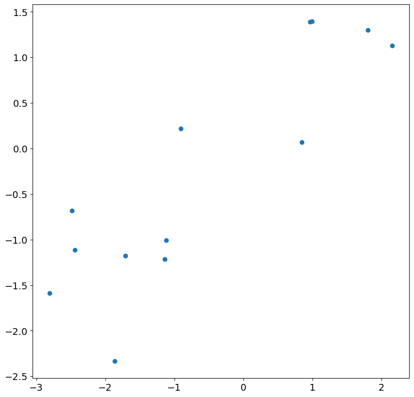
我們首先檢查最初 13 個殘差,並繪製它們與模型中的實際衝擊的關係圖。雖然存在對應關係,但它相當微弱,並且相關性遠小於 1。
[35]:
import matplotlib.pyplot as plt

plt.rc("figure", figsize=(10, 10))
plt.rc("font", size=14)

_ = plt.scatter(res.resid[:13], eta[200 : 200 + 13])
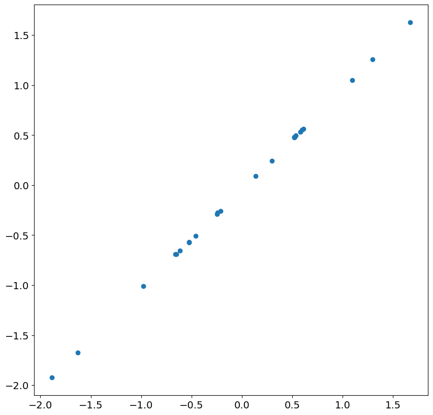
查看接下來 24 個殘差和衝擊,我們發現存在近乎完美的相關性。一旦忽略不太準確的殘差,這在大樣本中是預期的。
[36]:
_ = plt.scatter(res.resid[13:37], eta[200 + 13 : 200 + 37])
接下來,我們模擬一個 ARIMA(1,1,0),並包含時間趨勢。
[37]:
rng = np.random.default_rng(20210819)
eta = rng.standard_normal(5200)
rho = 0.8
beta = 20
epsilon = eta.copy()
for i in range(2, eta.shape[0]):
    epsilon[i] = (1 + rho) * epsilon[i - 1] - rho * epsilon[i - 2] + eta[i]
t = np.arange(epsilon.shape[0])
y = beta + 2 * t + epsilon
y = y[200:]
同樣,參數估計非常接近 DGP 參數。
[38]:
res = ARIMA(y, order=(1, 1, 0), trend="t").fit()
print(res.summary())
                               SARIMAX Results
==============================================================================
Dep. Variable:                      y   No. Observations:                 5000
Model:                 ARIMA(1, 1, 0)   Log Likelihood               -7067.739
Date:                Thu, 03 Oct 2024   AIC                          14141.479
Time:                        15:45:20   BIC                          14161.030
Sample:                             0   HQIC                         14148.331
                               - 5000
Covariance Type:                  opg
==============================================================================
                 coef    std err          z      P>|z|      [0.025      0.975]
------------------------------------------------------------------------------
x1             1.7747      0.069     25.642      0.000       1.639       1.910
ar.L1          0.7968      0.009     93.658      0.000       0.780       0.813
sigma2         0.9896      0.020     49.908      0.000       0.951       1.028
===================================================================================
Ljung-Box (L1) (Q):                   0.43   Jarque-Bera (JB):                 0.09
Prob(Q):                              0.51   Prob(JB):                         0.96
Heteroskedasticity (H):               0.97   Skew:                            -0.01
Prob(H) (two-sided):                  0.47   Kurtosis:                         2.99
===================================================================================

Warnings:
[1] Covariance matrix calculated using the outer product of gradients (complex-step).
殘差不準確,第一個殘差約為 500。其他殘差更接近,儘管在此模型中,通常應忽略前 2 個。
[39]:
res.resid[:5]
[39]:
array([ 5.08403002e+02, -1.58904197e+00, -1.54902446e+00,  1.04992617e-01,
        1.33644383e+00])
第一個殘差如此之大的原因是,此值的最佳預測是差值的平均值,即 1.77。一旦知道第一個值,第二個值就會在其預測中使用第一個值,並且預測值與真實值更接近。
[40]:
res.predict(0, 5)
[40]:
array([  1.77472562, 511.95355128, 510.87392196, 508.85708934,
       509.03356182, 511.85245439])
值得注意的是,結果類別包含兩個參數,它們可能有助於了解哪些殘差存在問題,即 loglikelihood_burn 和 nobs_diffuse。
[41]:
res.loglikelihood_burn, res.nobs_diffuse
[41]:
(1, 0)