TVP-VAR、MCMC 和稀疏模擬平滑
[1]:
%matplotlib inline

from importlib import reload
import numpy as np
import pandas as pd
import statsmodels.api as sm
import matplotlib.pyplot as plt

from scipy.stats import invwishart, invgamma

# Get the macro dataset
dta = sm.datasets.macrodata.load_pandas().data
dta.index = pd.date_range('1959Q1', '2009Q3', freq='QS')
背景
近年來,透過馬可夫鏈蒙地卡羅 (MCMC) 方法對線性高斯狀態空間模型進行貝氏分析已變得普遍且相對簡單,這尤其歸功於從資料和模型參數條件下的未觀測狀態向量聯合後驗分布中抽樣的進展(特別參見 Carter 和 Kohn (1994)、de Jong 和 Shephard (1995) 以及 Durbin 和 Koopman (2002))。這對於吉布斯抽樣 MCMC 方法特別有用。
雖然這些程序使用遞迴卡爾曼濾波器和平滑器的正向/反向應用,但另一項最近的研究採取不同的方法,並一次建構整個狀態向量的後驗聯合分布 - 特別參見 Chan 和 Jeliazkov (2009) 關於計量經濟時間序列處理,以及 McCausland 等人 (2011) 進行更全面的調查。特別是,後驗均值和精確矩陣會明確建構,而後者是一個稀疏帶狀矩陣。然後利用稀疏帶狀矩陣喬列斯基分解的有效演算法;這降低了記憶體成本,並可提高效能。依照 McCausland 等人 (2011) 的說法,我們將此方法稱為「喬列斯基因子演算法」(CFA) 方法。
與基於較常見的卡爾曼濾波器和平滑器 (KFS) 的模擬平滑器相比,基於 CFA 的模擬平滑器有一些優點和一些缺點。
CFA 的優點:
聯合後驗分布的推導相對簡單且易於理解。
在某些情況下,可能比 KFS 方法更快且記憶體消耗更少
在本筆記本結尾的附錄中,我們簡要討論了 TVP-VAR 模型兩種模擬平滑器的效能。總而言之:在單一機器上進行的簡單測試表明,對於 TVP-VAR 模型,Statsmodels 中的 CFA 和 KFS 實作具有大致相同的執行時間,而兩種實作的速度都比 Chan 和 Jeliazkov (2009) 提供的 Matlab 複寫程式碼快約兩倍。
CFA 的缺點:
主要缺點是此方法尚未(至少到目前為止)達到 KFS 方法的通用性。例如
它不能用於觀測或狀態方程式中具有降秩誤差項的模型。
這的一個含義是,在狀態方程式中包含恆等式以容納(例如)自迴歸模型中較高階滯後的典型狀態空間模型技巧不適用。這些模型仍然可以透過 CFA 方法處理,但代價是每個包含的滯後都需要稍微不同的實作。
例如,以狀態空間形式表示 ARMA 和 VARMA 過程的標準方法確實在觀測和/或狀態方程式中包含恆等式,因此 Chan 和 Jeliazkov (2009) 中提出的基本公式並未立即應用於這些模型。
狀態初始化/先驗的彈性較小。
在 Statsmodels 中的實作
已在 Statsmodels 中實作了類似於 Chan 和 Jeliazkov (2009) 中提出的基本公式的 CFA 模擬平滑器。
注意事項:
因此,Statsmodels 中的 CFA 模擬平滑器到目前為止僅支援狀態轉換確實是一階馬可夫過程的情況(即,它不支援已使用恆等式堆疊到一階過程的 p 階馬可夫過程)。
相反地,Statsmodels 中的 KFS 平滑器是完全通用的,可用於任何狀態空間模型,包括那些在觀測和狀態方程式中具有堆疊的 p 階馬可夫過程或其他恆等式的模型。
可以使用 simulation_smoother 方法從狀態空間模型建構 KFS 或 CFA 模擬平滑器。為了展示基本概念,我們先考慮一個簡單的範例。
局部水準模型
局部水準模型將觀測序列 \(y_t\) 分解為持久性趨勢 \(\mu_t\) 和暫時性誤差成分
此模型符合 CFA 模擬平滑器的要求,因為觀測誤差項 \(\varepsilon_t\) 和狀態創新項 \(\eta_t\) 都是非退化的 - 也就是說,它們的共變異數矩陣是滿秩的。
我們將此模型應用於通貨膨脹,並考慮從聯合狀態向量的後驗分佈中模擬繪製。也就是說,我們有興趣從以下分佈中取樣
其中我們定義 \(\mu^t \equiv (\mu_1, \dots, \mu_T)'\) 和 \(y^t \equiv (y_1, \dots, y_T)'\)。
在 Statsmodels 中,局部水準模型屬於更一般的「未觀測成分」模型類別,可以建構如下
[2]:
# Construct a local level model for inflation
mod = sm.tsa.UnobservedComponents(dta.infl, 'llevel')

# Fit the model's parameters (sigma2_varepsilon and sigma2_eta)
# via maximum likelihood
res = mod.fit()
print(res.params)

# Create simulation smoother objects
sim_kfs = mod.simulation_smoother()              # default method is KFS
sim_cfa = mod.simulation_smoother(method='cfa')  # can specify CFA method
RUNNING THE L-BFGS-B CODE

           * * *

Machine precision = 2.220D-16
 N =            2     M =           10

At X0         0 variables are exactly at the bounds

At iterate    0    f=  2.40814D+00    |proj g|=  1.27979D-01

At iterate    5    f=  2.24982D+00    |proj g|=  9.50561D-04

           * * *

Tit   = total number of iterations
Tnf   = total number of function evaluations
Tnint = total number of segments explored during Cauchy searches
Skip  = number of BFGS updates skipped
Nact  = number of active bounds at final generalized Cauchy point
Projg = norm of the final projected gradient
F     = final function value

           * * *

   N    Tit     Tnf  Tnint  Skip  Nact     Projg        F
    2      7      9      1     0     0   2.953D-07   2.250D+00
  F =   2.2498167187365663

CONVERGENCE: NORM_OF_PROJECTED_GRADIENT_<=_PGTOL
sigma2.irregular    3.373368
sigma2.level        0.744712
dtype: float64
This problem is unconstrained.
模擬平滑器物件 sim_kfs 和 sim_cfa 具有執行模擬平滑的 simulate 方法。每次呼叫 simulate 時,simulated_state 屬性將會使用從後驗中新模擬的繪圖重新填入。
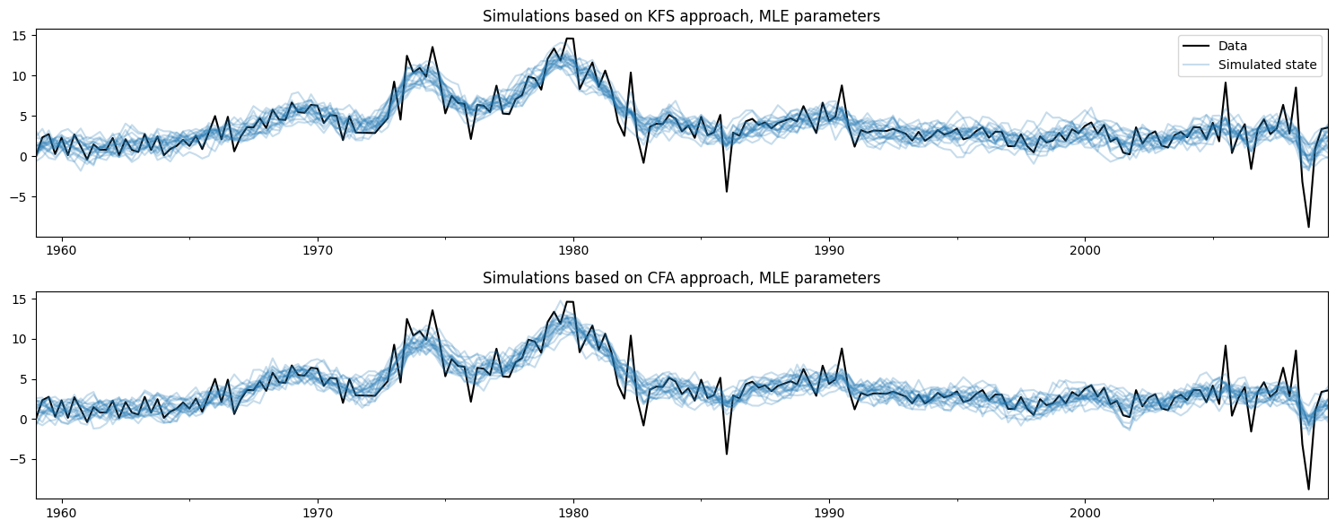
以下,我們使用 KFS 和 CFA 方法建構趨勢的 20 個模擬路徑,其中模擬是在最大概似參數估計下進行的。
[3]:
nsimulations = 20
simulated_state_kfs = pd.DataFrame(
    np.zeros((mod.nobs, nsimulations)), index=dta.index)
simulated_state_cfa = pd.DataFrame(
    np.zeros((mod.nobs, nsimulations)), index=dta.index)

for i in range(nsimulations):
    # Apply KFS simulation smoothing
    sim_kfs.simulate()
    # Save the KFS simulated state
    simulated_state_kfs.iloc[:, i] = sim_kfs.simulated_state[0]

    # Apply CFA simulation smoothing
    sim_cfa.simulate()
    # Save the CFA simulated state
    simulated_state_cfa.iloc[:, i] = sim_cfa.simulated_state[0]
繪製觀測資料和使用每種方法建立的模擬,不難看出這兩種方法正在做相同的事情。
[4]:
# Plot the inflation data along with simulated trends
fig, axes = plt.subplots(2, figsize=(15, 6))

# Plot data and KFS simulations
dta.infl.plot(ax=axes[0], color='k')
axes[0].set_title('Simulations based on KFS approach, MLE parameters')
simulated_state_kfs.plot(ax=axes[0], color='C0', alpha=0.25, legend=False)

# Plot data and CFA simulations
dta.infl.plot(ax=axes[1], color='k')
axes[1].set_title('Simulations based on CFA approach, MLE parameters')
simulated_state_cfa.plot(ax=axes[1], color='C0', alpha=0.25, legend=False)

# Add a legend, clean up layout
handles, labels = axes[0].get_legend_handles_labels()
axes[0].legend(handles[:2], ['Data', 'Simulated state'])
fig.tight_layout();
更新模型的參數
模擬平滑器與模型實例繫結,此處的變數為 mod。每當模型實例使用新參數更新時,模擬平滑器會在未來呼叫 simulate 方法時考慮到這些新參數。
這對於 MCMC 演算法很方便,該演算法會重複 (a) 更新模型的參數、(b) 繪製狀態向量的樣本,然後 (c) 繪製模型參數的新值。
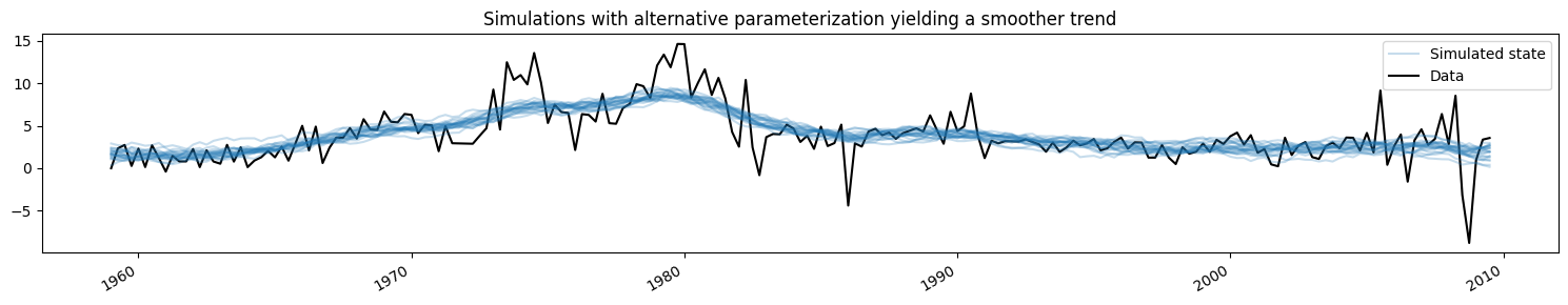
在這裡,我們會將模型更改為產生更平滑趨勢的不同參數化,並顯示模擬值如何變化(為了簡潔,我們只顯示來自 KFS 方法的模擬,但來自 CFA 方法的模擬會相同)。
[5]:
fig, ax = plt.subplots(figsize=(15, 3))

# Update the model's parameterization to one that attributes more
# variation in inflation to the observation error and so has less
# variation in the trend component
mod.update([4, 0.05])

# Plot simulations
for i in range(nsimulations):
    sim_kfs.simulate()
    ax.plot(dta.index, sim_kfs.simulated_state[0],
            color='C0', alpha=0.25, label='Simulated state')

# Plot data
dta.infl.plot(ax=ax, color='k', label='Data', zorder=-1)

# Add title, legend, clean up layout
ax.set_title('Simulations with alternative parameterization yielding a smoother trend')
handles, labels = ax.get_legend_handles_labels()
ax.legend(handles[-2:], labels[-2:])
fig.tight_layout();
應用:使用 MCMC 對 TVP-VAR 模型進行貝氏分析
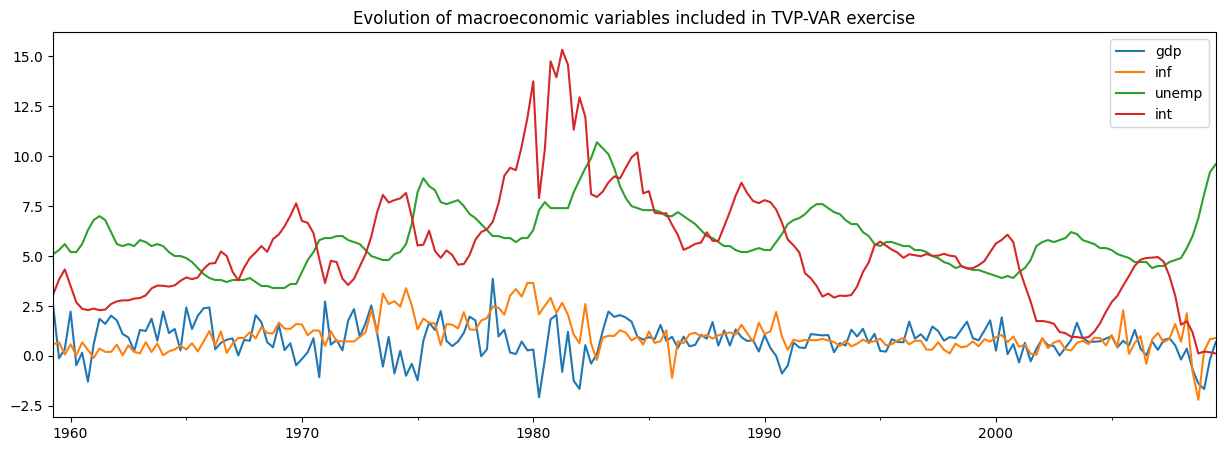
Chan 和 Jeliazkov (2009) 考慮的應用之一是時變參數向量自迴歸 (TVP-VAR) 模型,該模型使用貝氏吉布斯抽樣 (MCMC) 方法估計。他們將此應用於模擬四個總體經濟時間序列的共動性
實質 GDP 成長
通貨膨脹
失業率
短期利率
我們將使用 Statsmodels 中包含的非常相似的資料集來複寫他們的範例。
[6]:
# Subset to the four variables of interest
y = dta[['realgdp', 'cpi', 'unemp', 'tbilrate']].copy()
y.columns = ['gdp', 'inf', 'unemp', 'int']

# Convert to real GDP growth and CPI inflation rates
y[['gdp', 'inf']] = np.log(y[['gdp', 'inf']]).diff() * 100
y = y.iloc[1:]

fig, ax = plt.subplots(figsize=(15, 5))
y.plot(ax=ax)
ax.set_title('Evolution of macroeconomic variables included in TVP-VAR exercise');
TVP-VAR 模型
注意:本節基於 Chan 和 Jeliazkov (2009) 的第 3.1 節,您可以查閱該節以取得更多詳細資料。
通常的(時不變)VAR(1) 模型通常寫成
其中 \(y_t\) 是在時間 \(t\) 觀測到的 \(p \times 1\) 變數向量,而 \(H\) 是共變異數矩陣。
TVP-VAR(1) 模型將其推廣,允許係數根據時間變化。根據 \(\alpha_t = \text{vec}([\mu_t : \Phi_t])\) 將所有參數堆疊成一個向量,其中 \(\text{vec}\) 表示將矩陣的列堆疊成向量的操作,我們根據以下方式模擬它們隨時間的演變:
換句話說,每個參數都根據隨機漫步獨立演變。
請注意,\(\mu_t\) 中有 \(p\) 個係數,而 \(\Phi_t\) 中有 \(p^2\) 個係數,因此完整的狀態向量 \(\alpha\) 的形狀為 \(p * (p + 1) \times 1\)。
將 TVP-VAR(1) 模型放入狀態空間形式相對簡單,事實上我們只需要將觀察方程式重新寫成 SUR 形式即可
其中
只要 \(H\) 是滿秩的,並且每個變異數 \(\sigma_i^2\) 都非零,該模型就滿足 CFA 模擬平滑器的要求。
我們還需要為初始狀態 \(\alpha_1\) 指定初始化/先驗。這裡我們將遵循 Chan 和 Jeliazkov (2009) 的做法,使用 \(\alpha_1 \sim N(0, 5 I)\),儘管我們也可以將其建模為漫散的。
除了時變係數 \(\alpha_t\) 之外,我們還需要估計的其他參數是共變異數矩陣 \(H\) 和隨機漫步變異數 \(\sigma_i^2\) 中的項。
Statsmodels 中的 TVP-VAR 模型
在 Statsmodels 中以程式設計方式建構此模型也相對簡單,因為基本上有四個步驟
建立一個新的
TVPVAR類別作為sm.tsa.statespace.MLEModel的子類別填入狀態空間系統矩陣的固定值
指定 \(\alpha_1\) 的初始化
建立一個方法,用共變異數矩陣 \(H\) 和隨機漫步變異數 \(\sigma_i^2\) 的新值更新狀態空間系統矩陣。
為此,首先請注意 Statsmodels 使用的一般狀態空間表示形式為
然後 TVP-VAR(1) 模型暗示了以下專門化
截距項為零,即 \(c_t = d_t = 0\)
設計矩陣 \(Z_t\) 是時變的,但其值如上所述是固定的(即,其值包含 \(y_t\) 的 1 和滯後值)
觀察共變異數矩陣不是時變的,即 \(H_t = H_{t+1} = H\)
轉移矩陣不是時變的,並且等於單位矩陣,即 \(T_t = T_{t+1} = I\)
選擇矩陣 \(R_t\) 不是時變的,並且也等於單位矩陣,即 \(R_t = R_{t+1} = I\)
狀態共變異數矩陣 \(Q_t\) 不是時變的,並且是對角的,即 \(Q_t = Q_{t+1} = \text{diag}(\{\sigma_i^2\})\)
[7]:
# 1. Create a new TVPVAR class as a subclass of sm.tsa.statespace.MLEModel
class TVPVAR(sm.tsa.statespace.MLEModel):
    # Steps 2-3 are best done in the class "constructor", i.e. the __init__ method
    def __init__(self, y):
        # Create a matrix with [y_t' : y_{t-1}'] for t = 2, ..., T
        augmented = sm.tsa.lagmat(y, 1, trim='both', original='in', use_pandas=True)
        # Separate into y_t and z_t = [1 : y_{t-1}']
        p = y.shape[1]
        y_t = augmented.iloc[:, :p]
        z_t = sm.add_constant(augmented.iloc[:, p:])

        # Recall that the length of the state vector is p * (p + 1)
        k_states = p * (p + 1)
        super().__init__(y_t, exog=z_t, k_states=k_states)

        # Note that the state space system matrices default to contain zeros,
        # so we don't need to explicitly set c_t = d_t = 0.

        # Construct the design matrix Z_t
        # Notes:
        # -> self.k_endog = p is the dimension of the observed vector
        # -> self.k_states = p * (p + 1) is the dimension of the observed vector
        # -> self.nobs = T is the number of observations in y_t
        self['design'] = np.zeros((self.k_endog, self.k_states, self.nobs))
        for i in range(self.k_endog):
            start = i * (self.k_endog + 1)
            end = start + self.k_endog + 1
            self['design', i, start:end, :] = z_t.T

        # Construct the transition matrix T = I
        self['transition'] = np.eye(k_states)

        # Construct the selection matrix R = I
        self['selection'] = np.eye(k_states)

        # Step 3: Initialize the state vector as alpha_1 ~ N(0, 5I)
        self.ssm.initialize('known', stationary_cov=5 * np.eye(self.k_states))

    # Step 4. Create a method that we can call to update H and Q
    def update_variances(self, obs_cov, state_cov_diag):
        self['obs_cov'] = obs_cov
        self['state_cov'] = np.diag(state_cov_diag)

    # Finally, it can be convenient to define human-readable names for
    # each element of the state vector. These will be available in output
    @property
    def state_names(self):
        state_names = np.empty((self.k_endog, self.k_endog + 1), dtype=object)
        for i in range(self.k_endog):
            endog_name = self.endog_names[i]
            state_names[i] = (
                ['intercept.%s' % endog_name] +
                ['L1.%s->%s' % (other_name, endog_name) for other_name in self.endog_names])
        return state_names.ravel().tolist()
上面的類別定義了任何給定數據集的狀態空間模型。現在,我們需要使用我們先前建立的數據集(包含實際 GDP 成長率、通貨膨脹、失業率和利率)建立它的特定實例。
[8]:
# Create an instance of our TVPVAR class with our observed dataset y
mod = TVPVAR(y)
使用 H、Q 中的臨時參數進行初步研究
在我們下面的分析中,我們需要以一些初始參數化開始我們的 MCMC 迭代。遵循 Chan 和 Jeliazkov (2009) 的做法,我們將 \(H\) 設定為我們數據集的樣本共變異數矩陣,並將每個 \(i\) 的 \(\sigma_i^2 = 0.01\)。
在討論允許我們對模型進行推論的 MCMC 方案之前,首先我們可以考慮在簡單地插入這些初始參數時模型的輸出。為了填入這些參數,我們使用我們先前定義的 update_variances 方法,然後在這些參數的條件下執行卡爾曼濾波和平滑。
警告:此練習僅為了解釋說明 - 我們必須等待 MCMC 練習的輸出,才能以有意義的方式研究模型的實際影響.
[9]:
initial_obs_cov = np.cov(y.T)
initial_state_cov_diag = [0.01] * mod.k_states

# Update H and Q
mod.update_variances(initial_obs_cov, initial_state_cov_diag)

# Perform Kalman filtering and smoothing
# (the [] is just an empty list that in some models might contain
# additional parameters. Here, we don't have any additional parameters
# so we just pass an empty list)
initial_res = mod.smooth([])
initial_res 變數包含在這些初始參數的條件下,卡爾曼濾波和平滑的輸出。特別是,我們可能對「平滑狀態」感興趣,即 \(E[\alpha_t \mid y^t, H, \{\sigma_i^2\}]\)。
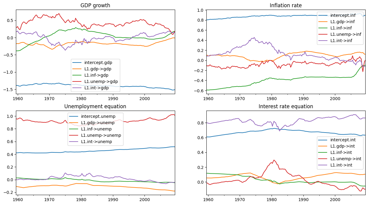
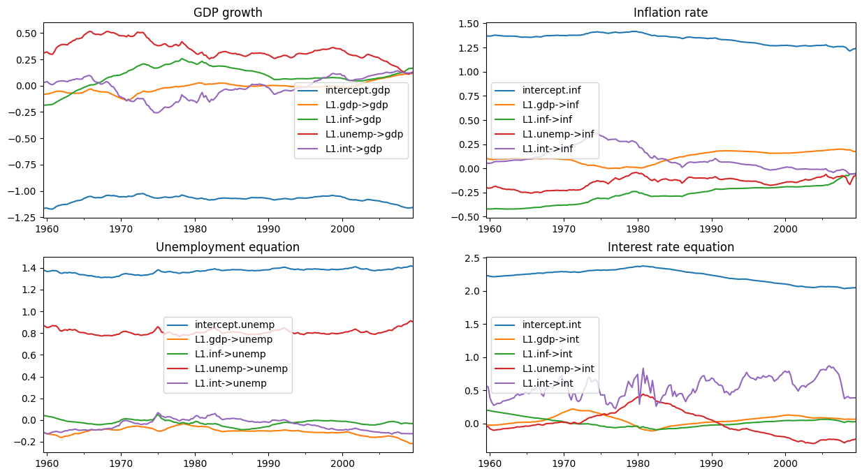
首先,讓我們建立一個函數,繪製係數隨時間變化的圖表,並將其區分為觀察變數方程式的方程式。
[10]:
def plot_coefficients_by_equation(states):
    fig, axes = plt.subplots(2, 2, figsize=(15, 8))

    # The way we defined Z_t implies that the first 5 elements of the
    # state vector correspond to the first variable in y_t, which is GDP growth
    ax = axes[0, 0]
    states.iloc[:, :5].plot(ax=ax)
    ax.set_title('GDP growth')
    ax.legend()

    # The next 5 elements correspond to inflation
    ax = axes[0, 1]
    states.iloc[:, 5:10].plot(ax=ax)
    ax.set_title('Inflation rate')
    ax.legend();

    # The next 5 elements correspond to unemployment
    ax = axes[1, 0]
    states.iloc[:, 10:15].plot(ax=ax)
    ax.set_title('Unemployment equation')
    ax.legend()

    # The last 5 elements correspond to the interest rate
    ax = axes[1, 1]
    states.iloc[:, 15:20].plot(ax=ax)
    ax.set_title('Interest rate equation')
    ax.legend();

    return ax
現在,我們對平滑狀態感興趣,這些狀態可在我們的結果物件 initial_res 中的 states.smoothed 屬性中找到。
如下圖所示,初始參數化表示某些係數存在顯著的時間變化。
[11]:
# Here, for illustration purposes only, we plot the time-varying
# coefficients conditional on an ad-hoc parameterization

# Recall that `initial_res` contains the Kalman filtering and smoothing,
# and the `states.smoothed` attribute contains the smoothed states
plot_coefficients_by_equation(initial_res.states.smoothed);
透過 MCMC 進行貝氏估計
我們現在將實作 Chan 和 Jeliazkov (2009) 演算法 2 中描述的吉布斯取樣器方案。
我們使用以下(條件共軛)先驗
其中 \(\mathcal{IW}\) 表示反向威沙特分布,而 \(\mathcal{IG}\) 表示反向伽瑪分布。我們將先驗超參數設定為
[12]:
# Prior hyperparameters

# Prior for obs. cov. is inverse-Wishart(v_1^0=k + 3, S10=I)
v10 = mod.k_endog + 3
S10 = np.eye(mod.k_endog)

# Prior for state cov. variances is inverse-Gamma(v_{i2}^0 / 2 = 3, S+{i2}^0 / 2 = 0.005)
vi20 = 6
Si20 = 0.01
在執行 MCMC 迭代之前,有幾個實際步驟
建立陣列來儲存我們狀態向量、觀察共變異數矩陣和狀態誤差變異數的繪圖。
將 H 和 Q 的初始值(如上所述)放入儲存向量
建構與我們的
TVPVAR實例相關聯的模擬平滑器物件,以繪製狀態向量的繪圖
[13]:
# Gibbs sampler setup
niter = 11000
nburn = 1000

# 1. Create storage arrays
store_states = np.zeros((niter + 1, mod.nobs, mod.k_states))
store_obs_cov = np.zeros((niter + 1, mod.k_endog, mod.k_endog))
store_state_cov = np.zeros((niter + 1, mod.k_states))

# 2. Put in the initial values
store_obs_cov[0] = initial_obs_cov
store_state_cov[0] = initial_state_cov_diag
mod.update_variances(store_obs_cov[0], store_state_cov[0])

# 3. Construct posterior samplers
sim = mod.simulation_smoother(method='cfa')
和之前一樣,我們可以使用基於卡爾曼濾波器和平滑器或基於喬列斯基因式分解演算法的模擬平滑器。
[14]:
for i in range(niter):
    mod.update_variances(store_obs_cov[i], store_state_cov[i])
    sim.simulate()

    # 1. Sample states
    store_states[i + 1] = sim.simulated_state.T

    # 2. Simulate obs cov
    fitted = np.matmul(mod['design'].transpose(2, 0, 1), store_states[i + 1][..., None])[..., 0]
    resid = mod.endog - fitted
    store_obs_cov[i + 1] = invwishart.rvs(v10 + mod.nobs, S10 + resid.T @ resid)

    # 3. Simulate state cov variances
    resid = store_states[i + 1, 1:] - store_states[i + 1, :-1]
    sse = np.sum(resid**2, axis=0)

    for j in range(mod.k_states):
        rv = invgamma.rvs((vi20 + mod.nobs - 1) / 2, scale=(Si20 + sse[j]) / 2)
        store_state_cov[i + 1, j] = rv
在刪除一些初始繪圖後,剩餘的後驗繪圖允許我們進行推論。下面,我們繪製時變迴歸係數的後驗平均值。
(注意:這些圖與 Chan 和 Jeliazkov (2009) 已出版版本中的圖 1 不同,但它們與 http://joshuachan.org/code/code_TVPVAR.html 提供的 Matlab 複製程式碼產生的圖非常相似。)
[15]:
# Collect the posterior means of each time-varying coefficient
states_posterior_mean = pd.DataFrame(
    np.mean(store_states[nburn + 1:], axis=0),
    index=mod._index, columns=mod.state_names)

# Plot these means over time
plot_coefficients_by_equation(states_posterior_mean);
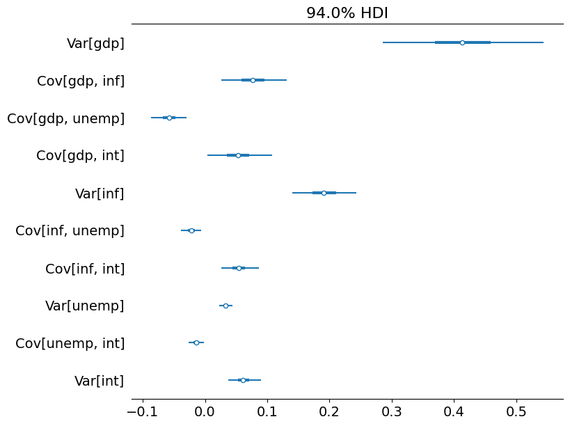
Python 還有許多程式庫可以協助探索貝氏模型。在這裡,我們將僅使用 arviz 套件來探索每個共變異數和變異數參數的可信區間,儘管它提供了更廣泛的分析工具集。
[16]:
import arviz as az

# Collect the observation error covariance parameters
az_obs_cov = az.convert_to_inference_data({
    ('Var[%s]' % mod.endog_names[i] if i == j else
     'Cov[%s, %s]' % (mod.endog_names[i], mod.endog_names[j])):
    store_obs_cov[nburn + 1:, i, j]
    for i in range(mod.k_endog) for j in range(i, mod.k_endog)})

# Plot the credible intervals
az.plot_forest(az_obs_cov, figsize=(8, 7));
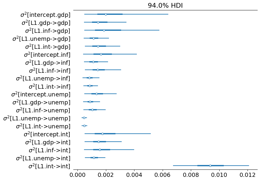
[17]:
# Collect the state innovation variance parameters
az_state_cov = az.convert_to_inference_data({
    r'$\sigma^2$[%s]' % mod.state_names[i]: store_state_cov[nburn + 1:, i]
    for i in range(mod.k_states)})

# Plot the credible intervals
az.plot_forest(az_state_cov, figsize=(8, 7));
附錄:效能
最後,我們執行一些簡單的測試,透過使用 %timeit Jupyter Notebook 魔術指令來比較 KFS 和 CFA 模擬平滑器的效能。
一個需要注意的地方是,KFS 模擬平滑器可以產生各種超出後驗狀態向量模擬的輸出,並且這些額外的計算可能會使結果產生偏差。為了使結果具有可比性,我們將透過使用 simulation_output 參數告訴 KFS 模擬平滑器僅計算狀態的模擬。
[18]:
from statsmodels.tsa.statespace.simulation_smoother import SIMULATION_STATE

sim_cfa = mod.simulation_smoother(method='cfa')
sim_kfs = mod.simulation_smoother(simulation_output=SIMULATION_STATE)
然後,我們可以使用以下程式碼來執行基本的計時練習
%timeit -n 10000 -r 3 sim_cfa.simulate()
%timeit -n 10000 -r 3 sim_kfs.simulate()
在此測試的機器上,這產生了以下結果
2.06 ms ± 26.5 µs per loop (mean ± std. dev. of 3 runs, 10000 loops each)
2.02 ms ± 68.4 µs per loop (mean ± std. dev. of 3 runs, 10000 loops each)
這些結果表明,至少對於此模型而言,相對於 KFS 方法,CFA 方法沒有明顯的計算收益。但是,這並不能排除以下情況
Statsmodels 中 CFA 模擬平滑器的實作可能會進一步最佳化
CFA 方法可能僅對某些模型(例如,具有大量
endog變數的模型)顯示出改進
評估第一個可能性的第一步簡單方法是,將 Statsmodels 中 CFA 模擬平滑器的執行時間與 Chan 和 Jeliazkov (2009) 複製程式碼中的 Matlab 實作進行比較,這些程式碼可於 http://joshuachan.org/code/code_TVPVAR.html 取得。
儘管 Statsmodels 版本的 CFA 模擬平滑器是用 Cython 編寫並編譯為 C 程式碼,但 Matlab 版本利用了 Matlab 的稀疏矩陣功能。因此,儘管它不是編譯的程式碼,我們可能會預期它具有相對良好的效能。
在此測試的機器上,Matlab 版本通常在 70-75 秒內執行具有 11,000 次迭代的 MCMC 迴圈,而此筆記本中使用 Statsmodels CFA 模擬平滑器(請參閱上文)的 MCMC 迴圈,也具有 11,000 次迭代,則在 40-45 秒內執行。這是一些證據表明 Statsmodels 的 CFA 平滑器實作已經表現相對良好(儘管它並未排除可能會有額外的收益)。
參考文獻
Carter, Chris K., and Robert Kohn. “On Gibbs sampling for state space models.” Biometrika 81, no. 3 (1994): 541-553.
Chan, Joshua CC, and Ivan Jeliazkov. “Efficient simulation and integrated likelihood estimation in state space models.” International Journal of Mathematical Modelling and Numerical Optimisation 1, no. 1-2 (2009): 101-120.
De Jong, Piet, and Neil Shephard. “The simulation smoother for time series models.” Biometrika 82, no. 2 (1995): 339-350.
Durbin, James, and Siem Jan Koopman. “A simple and efficient simulation smoother for state space time series analysis.” Biometrika 89, no. 3 (2002): 603-616.
McCausland, William J., Shirley Miller, and Denis Pelletier. “Simulation smoothing for state–space models: A computational efficiency analysis.” Computational Statistics & Data Analysis 55, no. 1 (2011): 199-212.