在狀態空間模型中估計或指定參數
在本筆記本中,我們展示如何在估計其他參數的同時,固定 statsmodels 狀態空間模型中某些參數的特定值。
一般而言,狀態空間模型允許使用者
透過最大似然估計所有參數
固定某些參數並估計其餘參數
固定所有參數(使不估計任何參數)
[1]:
%matplotlib inline

from importlib import reload
import numpy as np
import pandas as pd
import statsmodels.api as sm
import matplotlib.pyplot as plt

from pandas_datareader.data import DataReader
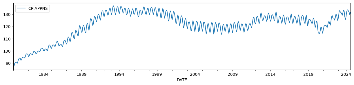
為了說明,我們將使用服裝的消費者物價指數,該指數具有隨時間變化的水平和強烈的季節性成分。
[2]:
endog = DataReader('CPIAPPNS', 'fred', start='1980').asfreq('MS')
endog.plot(figsize=(15, 3));
眾所周知(例如,Harvey 和 Jaeger [1993]),HP 濾波器的輸出可以由未觀察到的成分模型產生,只要對參數施加某些限制。
未觀察到的成分模型為
為了使趨勢與 HP 濾波器的輸出相匹配,必須按如下方式設定參數
其中 \(\lambda\) 是關聯的 HP 濾波器的參數。對於我們在此使用的每月數據,通常建議使用 \(\lambda = 129600\)。
[3]:
# Run the HP filter with lambda = 129600
hp_cycle, hp_trend = sm.tsa.filters.hpfilter(endog, lamb=129600)

# The unobserved components model above is the local linear trend, or "lltrend", specification
mod = sm.tsa.UnobservedComponents(endog, 'lltrend')
print(mod.param_names)
['sigma2.irregular', 'sigma2.level', 'sigma2.trend']
未觀察到的成分模型 (UCM) 的參數寫為
\(\sigma_\varepsilon^2 = \text{sigma2.irregular}\)
\(\sigma_\eta^2 = \text{sigma2.level}\)
\(\sigma_\zeta^2 = \text{sigma2.trend}\)
為了滿足上述限制,我們將設定 \((\sigma_\varepsilon^2, \sigma_\eta^2, \sigma_\zeta^2) = (1, 0, 1 / 129600)\)。
由於我們在此固定所有參數,因此完全不需要使用 fit 方法,因為該方法用於執行最大似然估計。相反,我們可以透過使用 smooth 方法,直接在我們選擇的參數下執行 Kalman 濾波器和平滑器。
[4]:
res = mod.smooth([1., 0, 1. / 129600])
print(res.summary())
                        Unobserved Components Results
==============================================================================
Dep. Variable:               CPIAPPNS   No. Observations:                  536
Model:             local linear trend   Log Likelihood               -2997.309
Date:                Thu, 03 Oct 2024   AIC                           6000.619
Time:                        15:45:23   BIC                           6013.460
Sample:                    01-01-1980   HQIC                          6005.643
                         - 08-01-2024
Covariance Type:                  opg
====================================================================================
                       coef    std err          z      P>|z|      [0.025      0.975]
------------------------------------------------------------------------------------
sigma2.irregular     1.0000      0.009    115.621      0.000       0.983       1.017
sigma2.level              0      0.000          0      1.000      -0.000       0.000
sigma2.trend      7.716e-06   1.98e-07     38.962      0.000    7.33e-06     8.1e-06
===================================================================================
Ljung-Box (L1) (Q):                 254.28   Jarque-Bera (JB):                 1.58
Prob(Q):                              0.00   Prob(JB):                         0.45
Heteroskedasticity (H):               2.21   Skew:                             0.04
Prob(H) (two-sided):                  0.00   Kurtosis:                         2.75
===================================================================================

Warnings:
[1] Covariance matrix calculated using the outer product of gradients (complex-step).
與 HP 濾波器趨勢估計值相對應的估計值,由 level 的平滑估計值給出(在上面的符號中,即為 \(\mu_t\))
[5]:
ucm_trend = pd.Series(res.level.smoothed, index=endog.index)
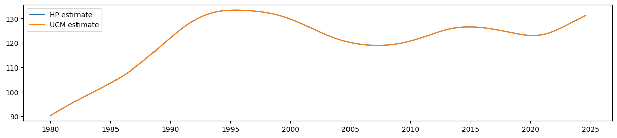
很容易看出,來自 UCM 的平滑水平估計值等於 HP 濾波器的輸出
[6]:
fig, ax = plt.subplots(figsize=(15, 3))

ax.plot(hp_trend, label='HP estimate')
ax.plot(ucm_trend, label='UCM estimate')
ax.legend();
加入季節性成分
然而,未觀察到的成分模型比 HP 濾波器更具彈性。例如,上面顯示的數據明顯具有季節性,但季節性影響隨時間變化(開始時的季節性比結束時弱得多)。未觀察到的成分架構的好處之一是,我們可以加入隨機季節性成分。在這種情況下,我們將透過最大似然估計季節性成分的變異數,同時仍包含上述參數上的限制,以便趨勢與 HP 濾波器的概念相對應。
加入隨機季節性成分會加入一個新參數 sigma2.seasonal。
[7]:
# Construct a local linear trend model with a stochastic seasonal component of period 1 year
mod = sm.tsa.UnobservedComponents(endog, 'lltrend', seasonal=12, stochastic_seasonal=True)
print(mod.param_names)
['sigma2.irregular', 'sigma2.level', 'sigma2.trend', 'sigma2.seasonal']
在這種情況下,我們將繼續如上所述限制前三個參數,但我們希望透過最大似然估計 sigma2.seasonal 的值。因此,我們將使用 fit 方法以及 fix_params 環境管理器。
fix_params 方法會接收參數名稱和關聯值的字典。在產生的環境中,這些參數將在所有情況下使用。在 fit 方法的情況下,只會估計未固定的參數。
[8]:
# Here we restrict the first three parameters to specific values
with mod.fix_params({'sigma2.irregular': 1, 'sigma2.level': 0, 'sigma2.trend': 1. / 129600}):
    # Now we fit any remaining parameters, which in this case
    # is just `sigma2.seasonal`
    res_restricted = mod.fit()
RUNNING THE L-BFGS-B CODE

           * * *

Machine precision = 2.220D-16
 N =            1     M =           10

At X0         0 variables are exactly at the bounds

At iterate    0    f=  3.87642D+00    |proj g|=  2.27476D-01

At iterate    5    f=  3.25868D+00    |proj g|=  2.20983D-06

           * * *

Tit   = total number of iterations
Tnf   = total number of function evaluations
Tnint = total number of segments explored during Cauchy searches
Skip  = number of BFGS updates skipped
Nact  = number of active bounds at final generalized Cauchy point
Projg = norm of the final projected gradient
F     = final function value

           * * *

   N    Tit     Tnf  Tnint  Skip  Nact     Projg        F
    1      5     12      1     0     0   2.210D-06   3.259D+00
  F =   3.2586810226319427

CONVERGENCE: NORM_OF_PROJECTED_GRADIENT_<=_PGTOL
This problem is unconstrained.
或者,我們也可以直接使用 fit_constrained 方法,該方法也接收約束字典
[9]:
res_restricted = mod.fit_constrained({'sigma2.irregular': 1, 'sigma2.level': 0, 'sigma2.trend': 1. / 129600})
RUNNING THE L-BFGS-B CODE

           * * *

Machine precision = 2.220D-16
 N =            1     M =           10

At X0         0 variables are exactly at the bounds

At iterate    0    f=  3.87642D+00    |proj g|=  2.27476D-01

At iterate    5    f=  3.25868D+00    |proj g|=  2.20983D-06

           * * *

Tit   = total number of iterations
Tnf   = total number of function evaluations
Tnint = total number of segments explored during Cauchy searches
Skip  = number of BFGS updates skipped
Nact  = number of active bounds at final generalized Cauchy point
Projg = norm of the final projected gradient
F     = final function value

           * * *

   N    Tit     Tnf  Tnint  Skip  Nact     Projg        F
    1      5     12      1     0     0   2.210D-06   3.259D+00
  F =   3.2586810226319427

CONVERGENCE: NORM_OF_PROJECTED_GRADIENT_<=_PGTOL
This problem is unconstrained.
摘要輸出包含所有參數,但指出前三個參數已固定(因此未進行估計)。
[10]:
print(res_restricted.summary())
                            Unobserved Components Results
=====================================================================================
Dep. Variable:                      CPIAPPNS   No. Observations:                  536
Model:                    local linear trend   Log Likelihood               -1746.653
                   + stochastic seasonal(12)   AIC                           3495.306
Date:                       Thu, 03 Oct 2024   BIC                           3499.566
Time:                               15:45:24   HQIC                          3496.974
Sample:                           01-01-1980
                                - 08-01-2024
Covariance Type:                         opg
============================================================================================
                               coef    std err          z      P>|z|      [0.025      0.975]
--------------------------------------------------------------------------------------------
sigma2.irregular (fixed)     1.0000        nan        nan        nan         nan         nan
sigma2.level (fixed)              0        nan        nan        nan         nan         nan
sigma2.trend (fixed)      7.716e-06        nan        nan        nan         nan         nan
sigma2.seasonal              0.0924      0.007     12.672      0.000       0.078       0.107
===================================================================================
Ljung-Box (L1) (Q):                 459.85   Jarque-Bera (JB):                38.49
Prob(Q):                              0.00   Prob(JB):                         0.00
Heteroskedasticity (H):               2.44   Skew:                             0.30
Prob(H) (two-sided):                  0.00   Kurtosis:                         4.19
===================================================================================

Warnings:
[1] Covariance matrix calculated using the outer product of gradients (complex-step).
為了進行比較,我們建構了不受限制的最大似然估計 (MLE)。在這種情況下,水平的估計值將不再對應於 HP 濾波器的概念。
[11]:
res_unrestricted = mod.fit()
RUNNING THE L-BFGS-B CODE

           * * *

Machine precision = 2.220D-16
 N =            4     M =           10

At X0         0 variables are exactly at the bounds

At iterate    0    f=  3.63596D+00    |proj g|=  1.07339D-01
This problem is unconstrained.
At iterate    5    f=  2.03169D+00    |proj g|=  4.05225D-01
  ys=-5.696E-01  -gs= 2.818E-01 BFGS update SKIPPED

At iterate   10    f=  1.59907D+00    |proj g|=  7.62230D-01

At iterate   15    f=  1.44540D+00    |proj g|=  2.77893D-01

At iterate   20    f=  1.39111D+00    |proj g|=  1.56723D-01

At iterate   25    f=  1.38688D+00    |proj g|=  1.41002D-03

           * * *

Tit   = total number of iterations
Tnf   = total number of function evaluations
Tnint = total number of segments explored during Cauchy searches
Skip  = number of BFGS updates skipped
Nact  = number of active bounds at final generalized Cauchy point
Projg = norm of the final projected gradient
F     = final function value

           * * *

   N    Tit     Tnf  Tnint  Skip  Nact     Projg        F
    4     28     58      1     1     0   2.548D-06   1.387D+00
  F =   1.3868826049230436

CONVERGENCE: NORM_OF_PROJECTED_GRADIENT_<=_PGTOL
最後,我們可以擷取趨勢和季節性成分的平滑估計值。
[12]:
# Construct the smoothed level estimates
unrestricted_trend = pd.Series(res_unrestricted.level.smoothed, index=endog.index)
restricted_trend = pd.Series(res_restricted.level.smoothed, index=endog.index)

# Construct the smoothed estimates of the seasonal pattern
unrestricted_seasonal = pd.Series(res_unrestricted.seasonal.smoothed, index=endog.index)
restricted_seasonal = pd.Series(res_restricted.seasonal.smoothed, index=endog.index)
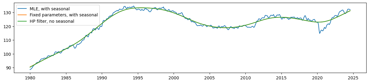
比較估計的水平,很明顯,具有固定參數的季節性 UCM 仍然會產生一個非常接近(雖然不再完全)HP 濾波器輸出的趨勢。
同時,來自沒有參數限制模型(MLE 模型)的估計水平比這些平滑得多。
[13]:
fig, ax = plt.subplots(figsize=(15, 3))

ax.plot(unrestricted_trend, label='MLE, with seasonal')
ax.plot(restricted_trend, label='Fixed parameters, with seasonal')
ax.plot(hp_trend, label='HP filter, no seasonal')
ax.legend();
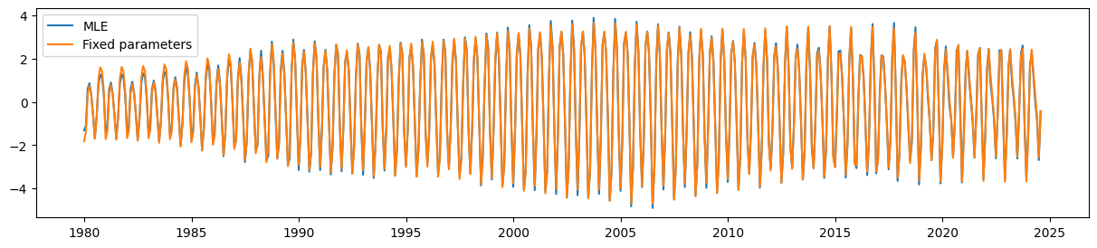
最後,具有參數限制的 UCM 仍然能夠很好地拾取隨時間變化的季節性成分。
[14]:
fig, ax = plt.subplots(figsize=(15, 3))

ax.plot(unrestricted_seasonal, label='MLE')
ax.plot(restricted_seasonal, label='Fixed parameters')
ax.legend();