SARIMAX:模型選擇,遺失數據
此範例仿效 Durbin 和 Koopman (2012) 第 8.4 章,應用 Box-Jenkins 方法來擬合 ARMA 模型。其新穎之處在於模型能夠處理具有遺失值的數據集。
[1]:
%matplotlib inline
[2]:
import numpy as np
import pandas as pd
from scipy.stats import norm
import statsmodels.api as sm
import matplotlib.pyplot as plt
[3]:
import requests
from io import BytesIO
from zipfile import ZipFile

# Download the dataset
df = pd.read_table(
    "https://raw.githubusercontent.com/jrnold/ssmodels-in-stan/master/StanStateSpace/data-raw/DK-data/internet.dat",
    skiprows=1, header=None, sep='\s+', engine='python',
    names=['internet','dinternet']
)
模型選擇
如同 Durbin 和 Koopman 所做,我們強制使一些值遺失。
[4]:
# Get the basic series
dta_full = df.dinternet[1:].values
dta_miss = dta_full.copy()

# Remove datapoints
missing = np.r_[6,16,26,36,46,56,66,72,73,74,75,76,86,96]-1
dta_miss[missing] = np.nan
然後,我們可以考慮使用赤池信息準則 (AIC) 進行模型選擇,但需要為每個變體執行模型,並選擇具有最低 AIC 值的模型。
這裡有幾點需要注意
當執行如此大量的模型時,尤其是在自迴歸和移動平均階數變大時,可能會出現不良的最大似然收斂。由於此範例僅為說明之用,因此我們忽略警告。
我們使用選項
enforce_invertibility=False,這允許移動平均多項式為不可逆,以便更多模型可估計。有幾個模型沒有產生良好的結果,其 AIC 值設為 NaN。這並不令人意外,因為 Durbin 和 Koopman 指出高階模型存在數值問題。
[5]:
import warnings

aic_full = pd.DataFrame(np.zeros((6,6), dtype=float))
aic_miss = pd.DataFrame(np.zeros((6,6), dtype=float))

warnings.simplefilter('ignore')

# Iterate over all ARMA(p,q) models with p,q in [0,6]
for p in range(6):
    for q in range(6):
        if p == 0 and q == 0:
            continue

        # Estimate the model with no missing datapoints
        mod = sm.tsa.statespace.SARIMAX(dta_full, order=(p,0,q), enforce_invertibility=False)
        try:
            res = mod.fit(disp=False)
            aic_full.iloc[p,q] = res.aic
        except:
            aic_full.iloc[p,q] = np.nan

        # Estimate the model with missing datapoints
        mod = sm.tsa.statespace.SARIMAX(dta_miss, order=(p,0,q), enforce_invertibility=False)
        try:
            res = mod.fit(disp=False)
            aic_miss.iloc[p,q] = res.aic
        except:
            aic_miss.iloc[p,q] = np.nan
對於在完整(非遺失)數據集上估計的模型,AIC 選擇 ARMA(1,1) 或 ARMA(3,0)。Durbin 和 Koopman 認為,由於簡潔性,ARMA(1,1) 規格更好。
\[\begin{split}\text{複製自:}\\ \textbf{表 8.1} ~~ \text{不同 ARMA 模型的 AIC。}\\ \newcommand{\r}[1]{{\color{red}{#1}}} \begin{array}{lrrrrrr} \hline q & 0 & 1 & 2 & 3 & 4 & 5 \\ \hline p & {} & {} & {} & {} & {} & {} \\ 0 & 0.00 & 549.81 & 519.87 & 520.27 & 519.38 & 518.86 \\ 1 & 529.24 & \r{514.30} & 516.25 & 514.58 & 515.10 & 516.28 \\ 2 & 522.18 & 516.29 & 517.16 & 515.77 & 513.24 & 514.73 \\ 3 & \r{511.99} & 513.94 & 515.92 & 512.06 & 513.72 & 514.50 \\ 4 & 513.93 & 512.89 & nan & nan & 514.81 & 516.08 \\ 5 & 515.86 & 517.64 & nan & nan & nan & nan \\ \hline \end{array}\end{split}\]
對於在遺失數據集上估計的模型,AIC 選擇 ARMA(1,1)
\[\begin{split}\text{複製自:}\\ \textbf{表 8.2} ~~ \text{具有遺失觀測值的不同 ARMA 模型的 AIC。}\\ \begin{array}{lrrrrrr} \hline q & 0 & 1 & 2 & 3 & 4 & 5 \\ \hline p & {} & {} & {} & {} & {} & {} \\ 0 & 0.00 & 488.93 & 464.01 & 463.86 & 462.63 & 463.62 \\ 1 & 468.01 & \r{457.54} & 459.35 & 458.66 & 459.15 & 461.01 \\ 2 & 469.68 & nan & 460.48 & 459.43 & 459.23 & 460.47 \\ 3 & 467.10 & 458.44 & 459.64 & 456.66 & 459.54 & 460.05 \\ 4 & 469.00 & 459.52 & nan & 463.04 & 459.35 & 460.96 \\ 5 & 471.32 & 461.26 & nan & nan & 461.00 & 462.97 \\ \hline \end{array}\end{split}\]
注意:AIC 值的計算方式與 Durbin 和 Koopman 不同,但總體趨勢相似。
估計後分析
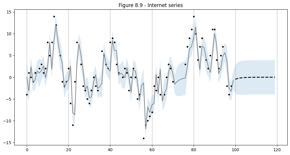
使用上面選擇的 ARMA(1,1) 規格,我們執行樣本內預測和樣本外預測。
[6]:
# Statespace
mod = sm.tsa.statespace.SARIMAX(dta_miss, order=(1,0,1))
res = mod.fit(disp=False)
print(res.summary())
                               SARIMAX Results
==============================================================================
Dep. Variable:                      y   No. Observations:                   99
Model:               SARIMAX(1, 0, 1)   Log Likelihood                -225.770
Date:                Thu, 03 Oct 2024   AIC                            457.541
Time:                        15:50:00   BIC                            465.326
Sample:                             0   HQIC                           460.691
                                 - 99
Covariance Type:                  opg
==============================================================================
                 coef    std err          z      P>|z|      [0.025      0.975]
------------------------------------------------------------------------------
ar.L1          0.6562      0.092      7.125      0.000       0.476       0.837
ma.L1          0.4878      0.111      4.390      0.000       0.270       0.706
sigma2        10.3402      1.569      6.591      0.000       7.265      13.415
===================================================================================
Ljung-Box (L1) (Q):                   0.00   Jarque-Bera (JB):                 1.87
Prob(Q):                              0.96   Prob(JB):                         0.39
Heteroskedasticity (H):               0.59   Skew:                            -0.10
Prob(H) (two-sided):                  0.13   Kurtosis:                         3.64
===================================================================================

Warnings:
[1] Covariance matrix calculated using the outer product of gradients (complex-step).
[7]:
# In-sample one-step-ahead predictions, and out-of-sample forecasts
nforecast = 20
predict = res.get_prediction(end=mod.nobs + nforecast)
idx = np.arange(len(predict.predicted_mean))
predict_ci = predict.conf_int(alpha=0.5)

# Graph
fig, ax = plt.subplots(figsize=(12,6))
ax.xaxis.grid()
ax.plot(dta_miss, 'k.')

# Plot
ax.plot(idx[:-nforecast], predict.predicted_mean[:-nforecast], 'gray')
ax.plot(idx[-nforecast:], predict.predicted_mean[-nforecast:], 'k--', linestyle='--', linewidth=2)
ax.fill_between(idx, predict_ci[:, 0], predict_ci[:, 1], alpha=0.15)

ax.set(title='Figure 8.9 - Internet series');
上次更新:2024 年 10 月 03 日