動態因素與同時指標
因素模型通常嘗試找出少數未觀察到的「因素」,這些因素會影響較多觀察到的變數中的大部分變異,並且與主成分分析等降維技術相關。動態因素模型明確地模擬了未觀察到的因素的轉移動態,因此通常應用於時間序列數據。
總體經濟同時指標旨在捕捉「商業週期」的共同組成部分;假設此組成部分會同時影響許多總體經濟變數。雖然同時指標的估計和使用(例如同時經濟指標指數)早於動態因素模型,但在幾篇有影響力的論文中,Stock 和 Watson(1989、1991)使用動態因素模型為它們提供了理論基礎。
以下,我們遵循 Kim 和 Nelson(1999)中發現的 Stock 和 Watson(1991)模型的處理方式,來制定動態因素模型,透過最大似然法估計其參數,並建立同時指標。
總體經濟數據
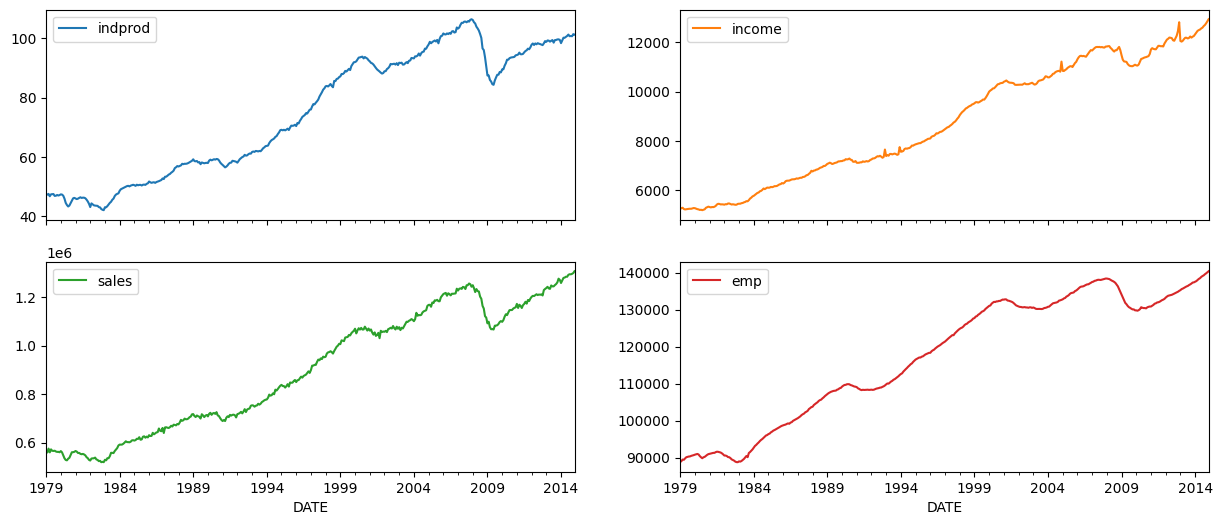
同時指標是透過考慮四個總體經濟變數的共同變動來建立的(這些變數的版本可在FRED上找到;下面使用的序列 ID 在括號中給出)
工業生產 (IPMAN)
實際總收入(不包括轉移支付)(W875RX1)
製造業和貿易銷售額 (CMRMTSPL)
非農業就業人數 (PAYEMS)
在所有情況下,數據都是按月頻率且已進行季節性調整;考慮的時間範圍是 1972 年至 2005 年。
[1]:
%matplotlib inline

import numpy as np
import pandas as pd
import statsmodels.api as sm
import matplotlib.pyplot as plt

np.set_printoptions(precision=4, suppress=True, linewidth=120)
[2]:
from pandas_datareader.data import DataReader

# Get the datasets from FRED
start = '1979-01-01'
end = '2014-12-01'
indprod = DataReader('IPMAN', 'fred', start=start, end=end)
income = DataReader('W875RX1', 'fred', start=start, end=end)
sales = DataReader('CMRMTSPL', 'fred', start=start, end=end)
emp = DataReader('PAYEMS', 'fred', start=start, end=end)
# dta = pd.concat((indprod, income, sales, emp), axis=1)
# dta.columns = ['indprod', 'income', 'sales', 'emp']
注意:在 FRED 最近的更新中(2015 年 8 月 12 日),時間序列 CMRMTSPL 被截斷為從 1997 年開始;這可能是由於 CMRMTSPL 是一個拼接序列的事實所導致的錯誤,因此早期期間來自序列 HMRMT,而後期期間由 CMRMT 定義。
此後(2016 年 2 月 11 日)已更正,但是也可以從 HMRMT 和 CMRMT 手動構建序列,如下所示(處理過程取自 Alfred xls 文件中的註解)。
[3]:
# HMRMT = DataReader('HMRMT', 'fred', start='1967-01-01', end=end)
# CMRMT = DataReader('CMRMT', 'fred', start='1997-01-01', end=end)
[4]:
# HMRMT_growth = HMRMT.diff() / HMRMT.shift()
# sales = pd.Series(np.zeros(emp.shape[0]), index=emp.index)

# # Fill in the recent entries (1997 onwards)
# sales[CMRMT.index] = CMRMT

# # Backfill the previous entries (pre 1997)
# idx = sales.loc[:'1997-01-01'].index
# for t in range(len(idx)-1, 0, -1):
#     month = idx[t]
#     prev_month = idx[t-1]
#     sales.loc[prev_month] = sales.loc[month] / (1 + HMRMT_growth.loc[prev_month].values)
[5]:
dta = pd.concat((indprod, income, sales, emp), axis=1)
dta.columns = ['indprod', 'income', 'sales', 'emp']
dta.index.freq = dta.index.inferred_freq
[6]:
dta.loc[:, 'indprod':'emp'].plot(subplots=True, layout=(2, 2), figsize=(15, 6));
Stock 和 Watson(1991)報告說,對於他們的數據集,他們無法拒絕每個序列中存在單位根的零假設(因此序列是積分的),但是他們沒有發現強有力的證據表明這些序列是協整的。
因此,他們建議使用變數的對數的一階差分來估計模型,並進行去平均和標準化。
[7]:
# Create log-differenced series
dta['dln_indprod'] = (np.log(dta.indprod)).diff() * 100
dta['dln_income'] = (np.log(dta.income)).diff() * 100
dta['dln_sales'] = (np.log(dta.sales)).diff() * 100
dta['dln_emp'] = (np.log(dta.emp)).diff() * 100

# De-mean and standardize
dta['std_indprod'] = (dta['dln_indprod'] - dta['dln_indprod'].mean()) / dta['dln_indprod'].std()
dta['std_income'] = (dta['dln_income'] - dta['dln_income'].mean()) / dta['dln_income'].std()
dta['std_sales'] = (dta['dln_sales'] - dta['dln_sales'].mean()) / dta['dln_sales'].std()
dta['std_emp'] = (dta['dln_emp'] - dta['dln_emp'].mean()) / dta['dln_emp'].std()
動態因素
一般動態因素模型寫為
其中 \(y_t\) 是觀察到的數據,\(f_t\) 是未觀察到的因素(作為向量自迴歸演進),\(x_t\) 是(可選)外生變數,而 \(u_t\) 是誤差或「特質」過程(\(u_t\) 也可選擇允許自相關)。 \(\Lambda\) 矩陣通常稱為「因素負載」矩陣。 因素誤差項的變異數設定為單位矩陣,以確保識別未觀察到的因素。
此模型可以轉換為狀態空間形式,並且可以透過卡爾曼濾波器估計未觀察到的因素。 可以將似然值評估為濾波遞迴的副產品,並且可以使用最大似然估計來估計參數。
模型規範
此應用中的特定動態因素模型具有 1 個未觀察到的因素,假設該因素遵循 AR(2) 過程。 假設創新 \(\varepsilon_t\) 是獨立的(因此 \(\Sigma\) 是對角矩陣),並且假設與每個方程式相關聯的誤差項 \(u_{i,t}\) 遵循獨立的 AR(2) 過程。
因此,這裡考慮的規範是
其中 \(i\) 是以下其中之一:[indprod, income, sales, emp ]。
可以使用 statsmodels 中內建的 DynamicFactor 模型來制定此模型。特別地,我們具有以下規範
k_factors = 1- (有 1 個未觀察到的因素)factor_order = 2- (它遵循 AR(2) 過程)error_var = False- (誤差演變為獨立的 AR 過程,而不是作為 VAR 聯合演變 - 請注意這是預設選項,因此在下面未指定)error_order = 2- (誤差是 2 階自相關的:即 AR(2) 過程)error_cov_type = 'diagonal'- (創新是不相關的;這又是預設值)
建立模型後,可以透過最大似然法估計參數;這是使用 fit() 方法完成的。
注意:回想一下,我們已經對數據進行了去平均和標準化;這對於解釋後面的結果非常重要。
附註:在其經驗範例中,Kim 和 Nelson (1999) 實際上考慮了一個略有不同的模型,其中允許就業變數也取決於該因素的滯後值 - 此模型不適合內建的 DynamicFactor 類別,但是可以透過使用子類別來實作所需的新參數和限制來容納它 - 請參閱下面的附錄 A。
參數估計
多變量模型可能具有相對大量的參數,並且可能難以從局部最小值中逃脫以找到最大化的似然值。 為了嘗試減輕此問題,我使用 Scipy 中可用的修改後的 Powell 方法(請參閱 minimize 文件以獲取更多資訊)執行初始最大化步驟(從模型定義的起始參數開始)。 然後將得到的參數用作標準 LBFGS 優化方法中的起始參數。
[8]:
# Get the endogenous data
endog = dta.loc['1979-02-01':, 'std_indprod':'std_emp']

# Create the model
mod = sm.tsa.DynamicFactor(endog, k_factors=1, factor_order=2, error_order=2)
initial_res = mod.fit(method='powell', disp=False)
res = mod.fit(initial_res.params, disp=False)
估計值
一旦模型被估計,我們就可以使用兩個組件進行分析或推論
估計的參數
估計的因素
參數
估計的參數可能有助於了解模型的含義,儘管在具有大量觀察到的變數和/或未觀察到的因素的模型中,它們可能難以解釋。
造成這種困難的一個原因是因素負載和未觀察到的因素之間的識別問題。 一個容易看到的識別問題是負載和因素的符號:反轉所有因素負載和未觀察到的因素的符號將產生一個與下面顯示的模型等效的模型。
在這裡,此模型中一個容易解釋的含義是未觀察到的因素的持久性:我們發現它表現出相當大的持久性。
[9]:
print(res.summary(separate_params=False))
                                             Statespace Model Results
=================================================================================================================
Dep. Variable:     ['std_indprod', 'std_income', 'std_sales', 'std_emp']   No. Observations:                  431
Model:                                 DynamicFactor(factors=1, order=2)   Log Likelihood               -1586.566
                                                          + AR(2) errors   AIC                           3209.133
Date:                                                   Thu, 03 Oct 2024   BIC                           3282.323
Time:                                                           16:05:06   HQIC                          3238.031
Sample:                                                       02-01-1979
                                                            - 12-01-2014
Covariance Type:                                                     opg
====================================================================================================
                                       coef    std err          z      P>|z|      [0.025      0.975]
----------------------------------------------------------------------------------------------------
loading.f1.std_indprod               0.5044      0.007     70.635      0.000       0.490       0.518
loading.f1.std_income                0.2313      0.021     10.956      0.000       0.190       0.273
loading.f1.std_sales                 0.2707      0.020     13.249      0.000       0.231       0.311
loading.f1.std_emp                   0.6354      0.011     56.890      0.000       0.613       0.657
sigma2.std_indprod                   0.0023   3.89e-05     59.178      0.000       0.002       0.002
sigma2.std_income                    0.8423      0.022     37.629      0.000       0.798       0.886
sigma2.std_sales                     0.7672      0.053     14.516      0.000       0.664       0.871
sigma2.std_emp                       0.0553      0.001     91.451      0.000       0.054       0.056
L1.f1.f1                             0.3455      0.024     14.605      0.000       0.299       0.392
L2.f1.f1                             0.4471      0.025     17.718      0.000       0.398       0.497
L1.e(std_indprod).e(std_indprod)    -1.9726      0.001  -3312.592      0.000      -1.974      -1.971
L2.e(std_indprod).e(std_indprod)    -1.0000   2.82e-06  -3.54e+05      0.000      -1.000      -1.000
L1.e(std_income).e(std_income)      -0.2412      0.019    -12.760      0.000      -0.278      -0.204
L2.e(std_income).e(std_income)      -0.1400      0.033     -4.202      0.000      -0.205      -0.075
L1.e(std_sales).e(std_sales)        -0.3118      0.043     -7.299      0.000      -0.396      -0.228
L2.e(std_sales).e(std_sales)        -0.0287      0.030     -0.958      0.338      -0.088       0.030
L1.e(std_emp).e(std_emp)             0.3580      0.009     40.009      0.000       0.340       0.376
L2.e(std_emp).e(std_emp)             0.4870      0.010     50.717      0.000       0.468       0.506
================================================================================================
Ljung-Box (L1) (Q):     nan, 0.15, 0.62, 6.97   Jarque-Bera (JB):   nan, 10067.99, 9.30, 4015.88
Prob(Q):                nan, 0.70, 0.43, 0.01   Prob(JB):                  nan, 0.00, 0.01, 0.00
Heteroskedasticity (H): nan, 4.25, 0.50, 0.37   Skew:                     nan, -0.91, 0.02, 1.12
Prob(H) (two-sided):    nan, 0.00, 0.00, 0.00   Kurtosis:                nan, 26.61, 3.72, 17.79
================================================================================================

Warnings:
[1] Covariance matrix calculated using the outer product of gradients (complex-step).
/opt/hostedtoolcache/Python/3.10.15/x64/lib/python3.10/site-packages/statsmodels/tsa/stattools.py:1431: RuntimeWarning: invalid value encountered in divide
  test_statistic = numer_squared_sum / denom_squared_sum
/opt/hostedtoolcache/Python/3.10.15/x64/lib/python3.10/site-packages/statsmodels/tsa/stattools.py:702: RuntimeWarning: invalid value encountered in divide
  acf = avf[: nlags + 1] / avf[0]
估計的因子
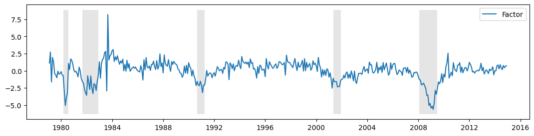
雖然繪製未觀察到的因子可能很有用,但在這裡它的用處不如人們想像的那麼大,原因有二:
上述與符號相關的識別問題。
由於數據經過差分處理,因此估計的因子解釋的是差分數據的變異,而不是原始數據的變異。
基於這些原因,我們創建了同時指標(coincident index,見下文)。
在這些保留意見下,我們將未觀察到的因子與美國經濟衰退的 NBER 指標一起繪製在下方。看起來該因子成功地捕捉到了一些商業週期活動的程度。
[10]:
fig, ax = plt.subplots(figsize=(13,3))

# Plot the factor
dates = endog.index._mpl_repr()
ax.plot(dates, res.factors.filtered[0], label='Factor')
ax.legend()

# Retrieve and also plot the NBER recession indicators
rec = DataReader('USREC', 'fred', start=start, end=end)
ylim = ax.get_ylim()
ax.fill_between(dates[:-3], ylim[0], ylim[1], rec.values[:-4,0], facecolor='k', alpha=0.1);
估計後
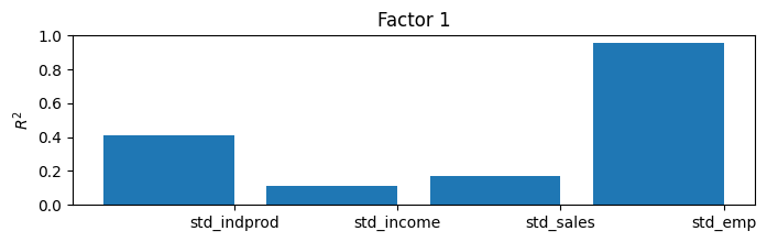
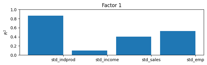
儘管在這裡我們可以通過構建同時指標來解釋模型結果,但有一種有用的通用方法可以了解估計因子正在捕捉什麼。通過將估計的因子視為給定值,將它們(以及常數)各自(一次一個)迴歸到每個觀察到的變量上,並記錄判定係數(\(R^2\) 值),我們可以了解每個因子解釋了很大一部分變異的變量,以及沒有解釋的變量。
在具有更多變量和更多因子的模型中,這有時可以幫助解釋這些因子(例如,有時一個因子主要影響實際變量,而另一個因子則影響名義變量)。
在這個只有四個內生變量和一個因子的模型中,很容易理解一個簡單的 \(R^2\) 值表,但在較大的模型中則不然。因此,通常會使用條形圖;從圖中我們可以清楚地看到,該因子解釋了工業生產指數的大部分變異,以及銷售和就業的很大一部分變異,但對於解釋收入的幫助較小。
[11]:
res.plot_coefficients_of_determination(figsize=(8,2));
同時指標
如上所述,該模型的目標是創建一個可解釋的序列,可以用於了解當前宏觀經濟的狀況。這就是同時指標旨在實現的目標。它在下面構建。對於想了解構建方法的讀者,請參閱 Kim 和 Nelson (1999) 或 Stock 和 Watson (1991)。
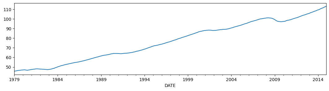
本質上,所做的是重建(差分)因子的平均值。我們將其與費城聯邦儲備銀行發布的同時指標(FRED 上的 USPHCI)進行比較。
[12]:
usphci = DataReader('USPHCI', 'fred', start='1979-01-01', end='2014-12-01')['USPHCI']
usphci.plot(figsize=(13,3));
[13]:
dusphci = usphci.diff()[1:].values
def compute_coincident_index(mod, res):
    # Estimate W(1)
    spec = res.specification
    design = mod.ssm['design']
    transition = mod.ssm['transition']
    ss_kalman_gain = res.filter_results.kalman_gain[:,:,-1]
    k_states = ss_kalman_gain.shape[0]

    W1 = np.linalg.inv(np.eye(k_states) - np.dot(
        np.eye(k_states) - np.dot(ss_kalman_gain, design),
        transition
    )).dot(ss_kalman_gain)[0]

    # Compute the factor mean vector
    factor_mean = np.dot(W1, dta.loc['1972-02-01':, 'dln_indprod':'dln_emp'].mean())

    # Normalize the factors
    factor = res.factors.filtered[0]
    factor *= np.std(usphci.diff()[1:]) / np.std(factor)

    # Compute the coincident index
    coincident_index = np.zeros(mod.nobs+1)
    # The initial value is arbitrary; here it is set to
    # facilitate comparison
    coincident_index[0] = usphci.iloc[0] * factor_mean / dusphci.mean()
    for t in range(0, mod.nobs):
        coincident_index[t+1] = coincident_index[t] + factor[t] + factor_mean

    # Attach dates
    coincident_index = pd.Series(coincident_index, index=dta.index).iloc[1:]

    # Normalize to use the same base year as USPHCI
    coincident_index *= (usphci.loc['1992-07-01'] / coincident_index.loc['1992-07-01'])

    return coincident_index
下面我們繪製了計算出的同時指標,以及美國經濟衰退和比較同時指標 USPHCI。
[14]:
fig, ax = plt.subplots(figsize=(13,3))

# Compute the index
coincident_index = compute_coincident_index(mod, res)

# Plot the factor
dates = endog.index._mpl_repr()
ax.plot(dates, coincident_index, label='Coincident index')
ax.plot(usphci.index._mpl_repr(), usphci, label='USPHCI')
ax.legend(loc='lower right')

# Retrieve and also plot the NBER recession indicators
ylim = ax.get_ylim()
ax.fill_between(dates[:-3], ylim[0], ylim[1], rec.values[:-4,0], facecolor='k', alpha=0.1);

附錄 1:擴展動態因子模型
回想一下,先前的規範由以下公式描述:
以狀態空間形式編寫,該模型的先前規範具有以下觀測方程式:
以及轉換方程式:
DynamicFactor 模型處理狀態空間表示的設置,並且在 DynamicFactor.update 方法中,它將擬合的參數值填入適當的位置。
擴展的規範與先前的示例相同,不同之處在於我們也希望允許就業取決於因子的滯後值。這會導致 \(y_{\text{emp},t}\) 方程式發生變化。現在我們有
現在,相應的觀測方程式應如下所示:
請注意,我們引入了兩個新的狀態變量,\(f_{t-2}\) 和 \(f_{t-3}\),這意味著我們需要更新轉換方程式:
這個模型無法直接由 DynamicFactor 類處理,但可以通過創建一個子類來處理,該子類以適當的方式更改狀態空間表示。
首先,請注意,如果我們設置 factor_order = 4,我們幾乎就能得到我們想要的結果。在這種情況下,觀測方程式的最後一行將是
而轉換方程式的第一行將是:
相對於我們想要的模型,我們有以下差異
在上述情況中,\(\lambda_{\text{emp}, j}\) 被強制設為零,當 \(j > 0\) 時,而我們希望它們能被估計為參數。
我們只希望因子根據 AR(2) 進行轉換,但在上述情況下,它是 AR(4)。
我們的策略將是子類化 DynamicFactor,並讓它完成大部分的工作(設定狀態空間表示等),其中它假設 factor_order = 4。我們在子類中實際要做的唯一事情是修正這兩個問題。
首先,這是子類的完整程式碼;將在下面討論。一開始就必須注意的是,下面定義的任何方法都不能省略。事實上,方法 __init__、 start_params、param_names、transform_params、untransform_params 和 update 構成了 statsmodels 中所有狀態空間模型的核心,而不僅僅是 DynamicFactor 類別。
[15]:
from statsmodels.tsa.statespace import tools
class ExtendedDFM(sm.tsa.DynamicFactor):
    def __init__(self, endog, **kwargs):
            # Setup the model as if we had a factor order of 4
            super(ExtendedDFM, self).__init__(
                endog, k_factors=1, factor_order=4, error_order=2,
                **kwargs)

            # Note: `self.parameters` is an ordered dict with the
            # keys corresponding to parameter types, and the values
            # the number of parameters of that type.
            # Add the new parameters
            self.parameters['new_loadings'] = 3

            # Cache a slice for the location of the 4 factor AR
            # parameters (a_1, ..., a_4) in the full parameter vector
            offset = (self.parameters['factor_loadings'] +
                      self.parameters['exog'] +
                      self.parameters['error_cov'])
            self._params_factor_ar = np.s_[offset:offset+2]
            self._params_factor_zero = np.s_[offset+2:offset+4]

    @property
    def start_params(self):
        # Add three new loading parameters to the end of the parameter
        # vector, initialized to zeros (for simplicity; they could
        # be initialized any way you like)
        return np.r_[super(ExtendedDFM, self).start_params, 0, 0, 0]

    @property
    def param_names(self):
        # Add the corresponding names for the new loading parameters
        #  (the name can be anything you like)
        return super(ExtendedDFM, self).param_names + [
            'loading.L%d.f1.%s' % (i, self.endog_names[3]) for i in range(1,4)]

    def transform_params(self, unconstrained):
            # Perform the typical DFM transformation (w/o the new parameters)
            constrained = super(ExtendedDFM, self).transform_params(
            unconstrained[:-3])

            # Redo the factor AR constraint, since we only want an AR(2),
            # and the previous constraint was for an AR(4)
            ar_params = unconstrained[self._params_factor_ar]
            constrained[self._params_factor_ar] = (
                tools.constrain_stationary_univariate(ar_params))

            # Return all the parameters
            return np.r_[constrained, unconstrained[-3:]]

    def untransform_params(self, constrained):
            # Perform the typical DFM untransformation (w/o the new parameters)
            unconstrained = super(ExtendedDFM, self).untransform_params(
                constrained[:-3])

            # Redo the factor AR unconstrained, since we only want an AR(2),
            # and the previous unconstrained was for an AR(4)
            ar_params = constrained[self._params_factor_ar]
            unconstrained[self._params_factor_ar] = (
                tools.unconstrain_stationary_univariate(ar_params))

            # Return all the parameters
            return np.r_[unconstrained, constrained[-3:]]

    def update(self, params, transformed=True, **kwargs):
        # Peform the transformation, if required
        if not transformed:
            params = self.transform_params(params)
        params[self._params_factor_zero] = 0

        # Now perform the usual DFM update, but exclude our new parameters
        super(ExtendedDFM, self).update(params[:-3], transformed=True, **kwargs)

        # Finally, set our new parameters in the design matrix
        self.ssm['design', 3, 1:4] = params[-3:]
所以我們剛剛做了什麼?
``__init__``
這裡重要的步驟是指定我們正在操作的基礎動態因子模型。特別是,如上所述,我們使用 factor_order=4 進行初始化,即使我們最終只會得到因子的 AR(2) 模型。我們還執行了一些與一般設定相關的任務。
``start_params``
start_params 在最佳化器中用作初始值。由於我們新增了三個新的參數,因此我們需要將它們傳入。如果我們沒有這樣做,最佳化器將使用預設的起始值,這些值將缺少三個元素。
``param_names``
param_names 用於許多地方,尤其是在結果類別中。下面我們得到一個完整結果摘要,只有在所有參數都有關聯名稱時,才有可能這樣做。
``transform_params`` 和 ``untransform_params``
最佳化器以不受約束的方式選擇可能的參數值。這通常是不希望的(例如,因為變異數不能為負),並且 transform_params 用於將最佳化器使用的不受約束的值轉換為適合模型的受約束的值。變異數項通常會平方(以強制它們為正),並且 AR 延遲係數通常會受到約束,以產生一個靜態模型。untransform_params 用於反向操作(這很重要,因為起始參數通常根據適合模型的值指定,我們需要先將它們轉換為適合最佳化器的參數,然後才能開始最佳化例程)。
即使我們不需要轉換或反轉換我們的新參數(在理論上,載荷可以採用任何值),我們仍然需要修改此函數,原因有二
DynamicFactor類別中的版本預期比我們現在少的 3 個參數。至少,我們需要處理這三個新參數。DynamicFactor類別中的版本將因子延遲係數約束為靜態,就像它是 AR(4) 模型一樣。由於我們實際上使用的是 AR(2) 模型,因此我們需要重新進行約束。我們也在此處將最後兩個自回歸係數設定為零。
``update``
我們需要指定新的 update 方法最重要的原因是,我們有三個新的參數需要放入狀態空間公式中。特別是,我們讓父類別 DynamicFactor.update 處理將所有參數(除了三個新的參數)放入狀態空間表示中,然後我們手動放入最後三個參數。
[16]:
# Create the model
extended_mod = ExtendedDFM(endog)
initial_extended_res = extended_mod.fit(maxiter=1000, disp=False)
extended_res = extended_mod.fit(initial_extended_res.params, method='nm', maxiter=1000)
print(extended_res.summary(separate_params=False))
Optimization terminated successfully.
         Current function value: 4.686378
         Iterations: 279
         Function evaluations: 479
                                             Statespace Model Results
=================================================================================================================
Dep. Variable:     ['std_indprod', 'std_income', 'std_sales', 'std_emp']   No. Observations:                  431
Model:                                 DynamicFactor(factors=1, order=4)   Log Likelihood               -2019.829
                                                          + AR(2) errors   AIC                           4085.658
Date:                                                   Thu, 03 Oct 2024   BIC                           4179.178
Time:                                                           16:08:10   HQIC                          4122.583
Sample:                                                       02-01-1979
                                                            - 12-01-2014
Covariance Type:                                                     opg
====================================================================================================
                                       coef    std err          z      P>|z|      [0.025      0.975]
----------------------------------------------------------------------------------------------------
loading.f1.std_indprod              -0.7064      0.036    -19.661      0.000      -0.777      -0.636
loading.f1.std_income               -0.2505      0.039     -6.460      0.000      -0.327      -0.175
loading.f1.std_sales                -0.4504      0.023    -19.252      0.000      -0.496      -0.405
loading.f1.std_emp                  -0.4117      0.038    -10.805      0.000      -0.486      -0.337
sigma2.std_indprod                   0.2338      0.045      5.156      0.000       0.145       0.323
sigma2.std_income                    0.8735      0.030     29.571      0.000       0.816       0.931
sigma2.std_sales                     0.5226      0.035     15.117      0.000       0.455       0.590
sigma2.std_emp                       0.2599      0.023     11.352      0.000       0.215       0.305
L1.f1.f1                             0.2845      0.054      5.300      0.000       0.179       0.390
L2.f1.f1                             0.3890      0.058      6.686      0.000       0.275       0.503
L3.f1.f1                                  0   3.92e-10          0      1.000   -7.68e-10    7.68e-10
L4.f1.f1                                  0   3.92e-10          0      1.000   -7.68e-10    7.68e-10
L1.e(std_indprod).e(std_indprod)    -0.2225      0.119     -1.864      0.062      -0.456       0.011
L2.e(std_indprod).e(std_indprod)    -0.1977      0.094     -2.098      0.036      -0.382      -0.013
L1.e(std_income).e(std_income)      -0.2009      0.023     -8.915      0.000      -0.245      -0.157
L2.e(std_income).e(std_income)      -0.0981      0.047     -2.099      0.036      -0.190      -0.006
L1.e(std_sales).e(std_sales)        -0.4842      0.047    -10.269      0.000      -0.577      -0.392
L2.e(std_sales).e(std_sales)        -0.2280      0.050     -4.543      0.000      -0.326      -0.130
L1.e(std_emp).e(std_emp)             0.2325      0.041      5.707      0.000       0.153       0.312
L2.e(std_emp).e(std_emp)             0.4893      0.049     10.044      0.000       0.394       0.585
loading.L1.f1.std_emp               -0.0824      0.037     -2.257      0.024      -0.154      -0.011
loading.L2.f1.std_emp               -0.0065      0.035     -0.185      0.854      -0.076       0.063
loading.L3.f1.std_emp               -0.1730      0.028     -6.094      0.000      -0.229      -0.117
=====================================================================================================
Ljung-Box (L1) (Q):     0.13, 0.01, 1.06, 4.34   Jarque-Bera (JB):   272.57, 10233.58, 25.49, 3815.68
Prob(Q):                0.72, 0.92, 0.30, 0.04   Prob(JB):                     0.00, 0.00, 0.00, 0.00
Heteroskedasticity (H): 0.75, 4.84, 0.44, 0.44   Skew:                        0.26, -0.98, 0.26, 0.78
Prob(H) (two-sided):    0.08, 0.00, 0.00, 0.00   Kurtosis:                   6.86, 26.79, 4.07, 17.49
=====================================================================================================

Warnings:
[1] Covariance matrix calculated using the outer product of gradients (complex-step).
[2] Covariance matrix is singular or near-singular, with condition number 7.43e+17. Standard errors may be unstable.
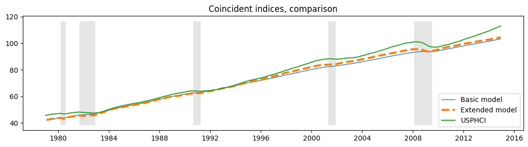
雖然此模型增加了似然性,但 AIC 和 BIC 指標不喜歡它,因為它們會懲罰額外的三個參數。
此外,定性結果沒有改變,正如我們從更新的 \(R^2\) 圖表和新的同步指標中看到的那樣,兩者實際上與先前的結果相同。
[17]:
extended_res.plot_coefficients_of_determination(figsize=(8,2));
[18]:
fig, ax = plt.subplots(figsize=(13,3))

# Compute the index
extended_coincident_index = compute_coincident_index(extended_mod, extended_res)

# Plot the factor
dates = endog.index._mpl_repr()
ax.plot(dates, coincident_index, '-', linewidth=1, label='Basic model')
ax.plot(dates, extended_coincident_index, '--', linewidth=3, label='Extended model')
ax.plot(usphci.index._mpl_repr(), usphci, label='USPHCI')
ax.legend(loc='lower right')
ax.set(title='Coincident indices, comparison')

# Retrieve and also plot the NBER recession indicators
ylim = ax.get_ylim()
ax.fill_between(dates[:-3], ylim[0], ylim[1], rec.values[:-4,0], facecolor='k', alpha=0.1);