時間序列資料中的季節性
考慮以多個具有不同週期性的季節性成分對時間序列資料進行建模的問題。讓我們取得時間序列 \(y_t\) 並明確地將其分解為一個水平成分和兩個季節性成分。
其中 \(\mu_t\) 代表趨勢或水平,\(\gamma^{(1)}_t\) 代表一個週期相對較短的季節性成分,而 \(\gamma^{(2)}_t\) 代表另一個週期較長的季節性成分。 我們將為我們的水平設定一個固定的截距項,並考慮 \(\gamma^{(2)}_t\) 和 \(\gamma^{(2)}_t\) 為隨機的,以便季節性模式可以隨時間變化。
在本筆記本中,我們將生成符合此模型的合成資料,並展示在未觀察到的成分建模框架下以幾種不同方式對季節性項進行建模。
[1]:
%matplotlib inline
[2]:
import numpy as np
import pandas as pd
import statsmodels.api as sm
import matplotlib.pyplot as plt

plt.rc("figure", figsize=(16,8))
plt.rc("font", size=14)
合成資料建立
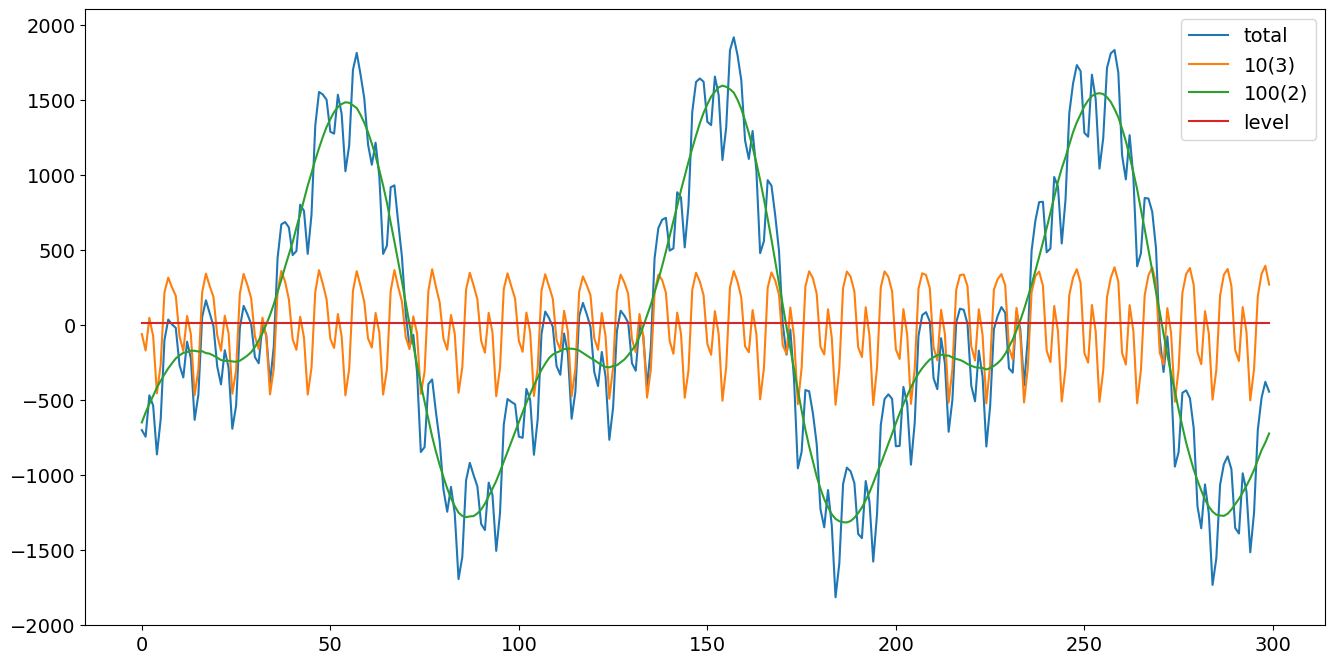
我們將按照 Durbin 和 Koopman (2012) 中的方程式 (3.7) 和 (3.8) 建立具有多個季節性模式的資料。我們將模擬 300 個週期和兩個在頻域中參數化的季節性項,其週期分別為 10 和 100,以及諧波數分別為 3 和 2。此外,它們隨機部分的變異數分別為 4 和 9。
[3]:
# First we'll simulate the synthetic data
def simulate_seasonal_term(periodicity, total_cycles, noise_std=1.,
                           harmonics=None):
    duration = periodicity * total_cycles
    assert duration == int(duration)
    duration = int(duration)
    harmonics = harmonics if harmonics else int(np.floor(periodicity / 2))

    lambda_p = 2 * np.pi / float(periodicity)

    gamma_jt = noise_std * np.random.randn((harmonics))
    gamma_star_jt = noise_std * np.random.randn((harmonics))

    total_timesteps = 100 * duration # Pad for burn in
    series = np.zeros(total_timesteps)
    for t in range(total_timesteps):
        gamma_jtp1 = np.zeros_like(gamma_jt)
        gamma_star_jtp1 = np.zeros_like(gamma_star_jt)
        for j in range(1, harmonics + 1):
            cos_j = np.cos(lambda_p * j)
            sin_j = np.sin(lambda_p * j)
            gamma_jtp1[j - 1] = (gamma_jt[j - 1] * cos_j
                                 + gamma_star_jt[j - 1] * sin_j
                                 + noise_std * np.random.randn())
            gamma_star_jtp1[j - 1] = (- gamma_jt[j - 1] * sin_j
                                      + gamma_star_jt[j - 1] * cos_j
                                      + noise_std * np.random.randn())
        series[t] = np.sum(gamma_jtp1)
        gamma_jt = gamma_jtp1
        gamma_star_jt = gamma_star_jtp1
    wanted_series = series[-duration:] # Discard burn in

    return wanted_series
[4]:
duration = 100 * 3
periodicities = [10, 100]
num_harmonics = [3, 2]
std = np.array([2, 3])
np.random.seed(8678309)

terms = []
for ix, _ in enumerate(periodicities):
    s = simulate_seasonal_term(
        periodicities[ix],
        duration / periodicities[ix],
        harmonics=num_harmonics[ix],
        noise_std=std[ix])
    terms.append(s)
terms.append(np.ones_like(terms[0]) * 10.)
series = pd.Series(np.sum(terms, axis=0))
df = pd.DataFrame(data={'total': series,
                        '10(3)': terms[0],
                        '100(2)': terms[1],
                        'level':terms[2]})
h1, = plt.plot(df['total'])
h2, = plt.plot(df['10(3)'])
h3, = plt.plot(df['100(2)'])
h4, = plt.plot(df['level'])
plt.legend(['total','10(3)','100(2)', 'level'])
plt.show()
未觀測到的成分 (頻域建模)
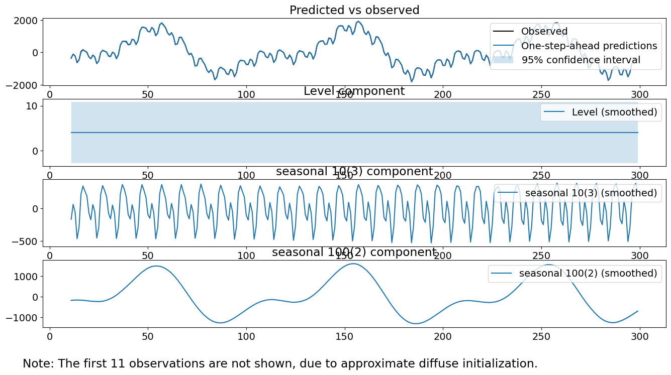
下一個方法是一個未觀測到的成分模型,其中趨勢被建模為一個固定的截距,而季節性成分則使用三角函數進行建模,其主要週期性分別為 10 和 100,諧波數分別為 3 和 2。請注意,這是正確的生成模型。時間序列的過程可以寫成
其中 \(\epsilon_t\) 是白雜訊,\(\omega^{(1)}_{j,t}\) 是獨立同分布的 \(N(0, \sigma^2_1)\),而 \(\omega^{(2)}_{j,t}\) 是獨立同分布的 \(N(0, \sigma^2_2)\),其中 \(\sigma_1 = 2.\)
[5]:
model = sm.tsa.UnobservedComponents(series.values,
                                    level='fixed intercept',
                                    freq_seasonal=[{'period': 10,
                                                    'harmonics': 3},
                                                   {'period': 100,
                                                    'harmonics': 2}])
res_f = model.fit(disp=False)
print(res_f.summary())
# The first state variable holds our estimate of the intercept
print("fixed intercept estimated as {0:.3f}".format(res_f.smoother_results.smoothed_state[0,-1:][0]))

res_f.plot_components()
plt.show()
                                Unobserved Components Results
==============================================================================================
Dep. Variable:                                      y   No. Observations:                  300
Model:                                fixed intercept   Log Likelihood               -1145.631
                    + stochastic freq_seasonal(10(3))   AIC                           2295.261
                   + stochastic freq_seasonal(100(2))   BIC                           2302.594
Date:                                Thu, 03 Oct 2024   HQIC                          2298.200
Time:                                        15:59:12
Sample:                                             0
                                                - 300
Covariance Type:                                  opg
===============================================================================================
                                  coef    std err          z      P>|z|      [0.025      0.975]
-----------------------------------------------------------------------------------------------
sigma2.freq_seasonal_10(3)      4.5942      0.565      8.126      0.000       3.486       5.702
sigma2.freq_seasonal_100(2)     9.7904      2.483      3.942      0.000       4.923      14.658
===================================================================================
Ljung-Box (L1) (Q):                   0.06   Jarque-Bera (JB):                 0.08
Prob(Q):                              0.81   Prob(JB):                         0.96
Heteroskedasticity (H):               1.17   Skew:                             0.01
Prob(H) (two-sided):                  0.45   Kurtosis:                         3.08
===================================================================================

Warnings:
[1] Covariance matrix calculated using the outer product of gradients (complex-step).
fixed intercept estimated as 4.053
[6]:
model.ssm.transition[:, :, 0]
[6]:
array([[ 1.        ,  0.        ,  0.        ,  0.        ,  0.        ,
         0.        ,  0.        ,  0.        ,  0.        ,  0.        ,
         0.        ],
       [ 0.        ,  0.80901699,  0.58778525,  0.        ,  0.        ,
         0.        ,  0.        ,  0.        ,  0.        ,  0.        ,
         0.        ],
       [ 0.        , -0.58778525,  0.80901699,  0.        ,  0.        ,
         0.        ,  0.        ,  0.        ,  0.        ,  0.        ,
         0.        ],
       [ 0.        ,  0.        ,  0.        ,  0.30901699,  0.95105652,
         0.        ,  0.        ,  0.        ,  0.        ,  0.        ,
         0.        ],
       [ 0.        ,  0.        ,  0.        , -0.95105652,  0.30901699,
         0.        ,  0.        ,  0.        ,  0.        ,  0.        ,
         0.        ],
       [ 0.        ,  0.        ,  0.        ,  0.        ,  0.        ,
        -0.30901699,  0.95105652,  0.        ,  0.        ,  0.        ,
         0.        ],
       [ 0.        ,  0.        ,  0.        ,  0.        ,  0.        ,
        -0.95105652, -0.30901699,  0.        ,  0.        ,  0.        ,
         0.        ],
       [ 0.        ,  0.        ,  0.        ,  0.        ,  0.        ,
         0.        ,  0.        ,  0.99802673,  0.06279052,  0.        ,
         0.        ],
       [ 0.        ,  0.        ,  0.        ,  0.        ,  0.        ,
         0.        ,  0.        , -0.06279052,  0.99802673,  0.        ,
         0.        ],
       [ 0.        ,  0.        ,  0.        ,  0.        ,  0.        ,
         0.        ,  0.        ,  0.        ,  0.        ,  0.9921147 ,
         0.12533323],
       [ 0.        ,  0.        ,  0.        ,  0.        ,  0.        ,
         0.        ,  0.        ,  0.        ,  0.        , -0.12533323,
         0.9921147 ]])
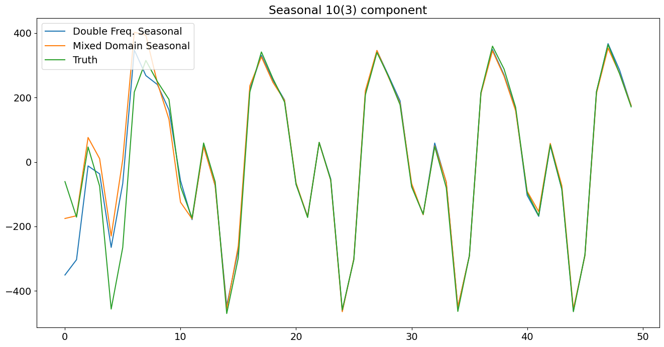
觀察到擬合的變異數與 4 和 9 的真實變異數非常接近。此外,個別的季節性成分看起來與真實的季節性成分非常接近。平滑後的水平項與真實水平 10 相當接近。最後,我們的診斷看起來很紮實;檢定統計量小到無法拒絕我們的三項檢定。
未觀測到的成分 (混合時域和頻域建模)
第二種方法是一個未觀測到的成分模型,其中趨勢被建模為一個固定的截距,而季節性成分則使用 10 個總和為 0 的常數和主要週期為 100 的三角函數進行建模,總共有 2 個諧波。請注意,這不是生成模型,因為它預設較短的季節性成分比實際情況有更多的狀態誤差。時間序列的過程可以寫成
其中 \(\epsilon_t\) 是白雜訊,\(\omega^{(1)}_{t}\) 是獨立同分布的 \(N(0, \sigma^2_1)\),而 \(\omega^{(2)}_{j,t}\) 是獨立同分布的 \(N(0, \sigma^2_2)\)。
[7]:
model = sm.tsa.UnobservedComponents(series,
                                    level='fixed intercept',
                                    seasonal=10,
                                    freq_seasonal=[{'period': 100,
                                                    'harmonics': 2}])
res_tf = model.fit(disp=False)
print(res_tf.summary())
# The first state variable holds our estimate of the intercept
print("fixed intercept estimated as {0:.3f}".format(res_tf.smoother_results.smoothed_state[0,-1:][0]))

fig = res_tf.plot_components()
fig.tight_layout(pad=1.0)
                                Unobserved Components Results
==============================================================================================
Dep. Variable:                                      y   No. Observations:                  300
Model:                                fixed intercept   Log Likelihood               -1238.113
                            + stochastic seasonal(10)   AIC                           2480.226
                   + stochastic freq_seasonal(100(2))   BIC                           2487.538
Date:                                Thu, 03 Oct 2024   HQIC                          2483.157
Time:                                        15:59:14
Sample:                                             0
                                                - 300
Covariance Type:                                  opg
===============================================================================================
                                  coef    std err          z      P>|z|      [0.025      0.975]
-----------------------------------------------------------------------------------------------
sigma2.seasonal                55.2934      7.114      7.773      0.000      41.351      69.236
sigma2.freq_seasonal_100(2)    28.6897      4.008      7.159      0.000      20.835      36.544
===================================================================================
Ljung-Box (L1) (Q):                  26.35   Jarque-Bera (JB):                 1.20
Prob(Q):                              0.00   Prob(JB):                         0.55
Heteroskedasticity (H):               1.27   Skew:                            -0.14
Prob(H) (two-sided):                  0.24   Kurtosis:                         2.87
===================================================================================

Warnings:
[1] Covariance matrix calculated using the outer product of gradients (complex-step).
fixed intercept estimated as 4.468
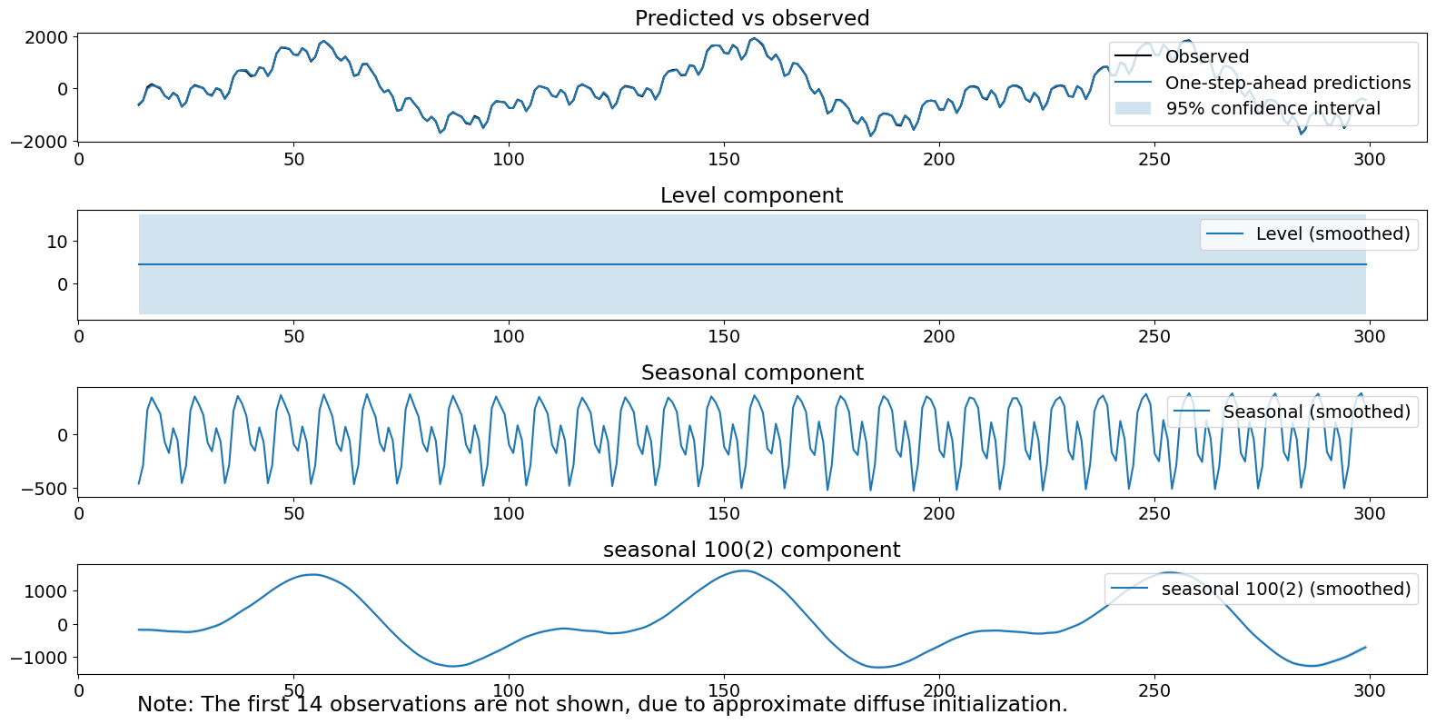
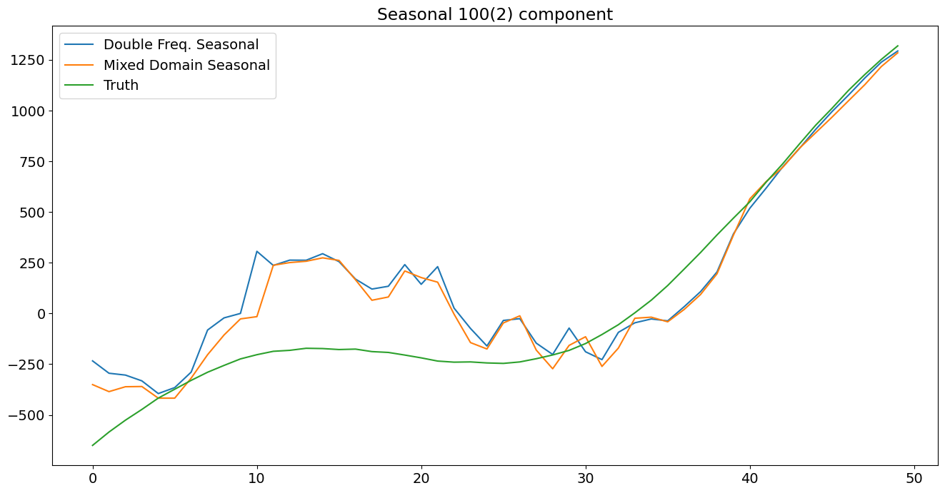
繪製的成分看起來不錯。然而,第二個季節性項的估計變異數從實際情況膨脹。此外,我們拒絕 Ljung-Box 統計量,表明在考慮我們的成分後,我們可能仍有自相關。
未觀測到的成分 (惰性頻域建模)
第三種方法是一個具有固定截距和一個季節性成分的未觀測到的成分模型,該成分使用主週期為 100 和 50 個諧波的三角函數進行建模。請注意,這不是生成模型,因為它預設比實際情況有更多的諧波。由於變異數是連繫在一起的,我們無法將不存在的諧波的估計共變數驅動為 0。此模型規格的惰性之處在於我們沒有費心指定兩個不同的季節性成分,而是選擇使用一個具有足夠諧波的單個成分對它們進行建模,以涵蓋兩者。我們將無法捕捉到兩個真實成分之間變異數的任何差異。時間序列的過程可以寫成
其中 \(\epsilon_t\) 是白雜訊,\(\omega^{(1)}_{t}\) 是獨立同分布的 \(N(0, \sigma^2_1)\)。
[8]:
model = sm.tsa.UnobservedComponents(series,
                                    level='fixed intercept',
                                    freq_seasonal=[{'period': 100}])
res_lf = model.fit(disp=False)
print(res_lf.summary())
# The first state variable holds our estimate of the intercept
print("fixed intercept estimated as {0:.3f}".format(res_lf.smoother_results.smoothed_state[0,-1:][0]))

fig = res_lf.plot_components()
fig.tight_layout(pad=1.0)
                                 Unobserved Components Results
===============================================================================================
Dep. Variable:                                       y   No. Observations:                  300
Model:                                 fixed intercept   Log Likelihood               -1101.455
                   + stochastic freq_seasonal(100(50))   AIC                           2204.910
Date:                                 Thu, 03 Oct 2024   BIC                           2208.204
Time:                                         16:06:42   HQIC                          2206.243
Sample:                                              0
                                                 - 300
Covariance Type:                                   opg
================================================================================================
                                   coef    std err          z      P>|z|      [0.025      0.975]
------------------------------------------------------------------------------------------------
sigma2.freq_seasonal_100(50)     0.7591      0.082      9.233      0.000       0.598       0.920
===================================================================================
Ljung-Box (L1) (Q):                  85.96   Jarque-Bera (JB):                 0.72
Prob(Q):                              0.00   Prob(JB):                         0.70
Heteroskedasticity (H):               1.00   Skew:                            -0.01
Prob(H) (two-sided):                  0.99   Kurtosis:                         2.71
===================================================================================

Warnings:
[1] Covariance matrix calculated using the outer product of gradients (complex-step).
fixed intercept estimated as 4.426
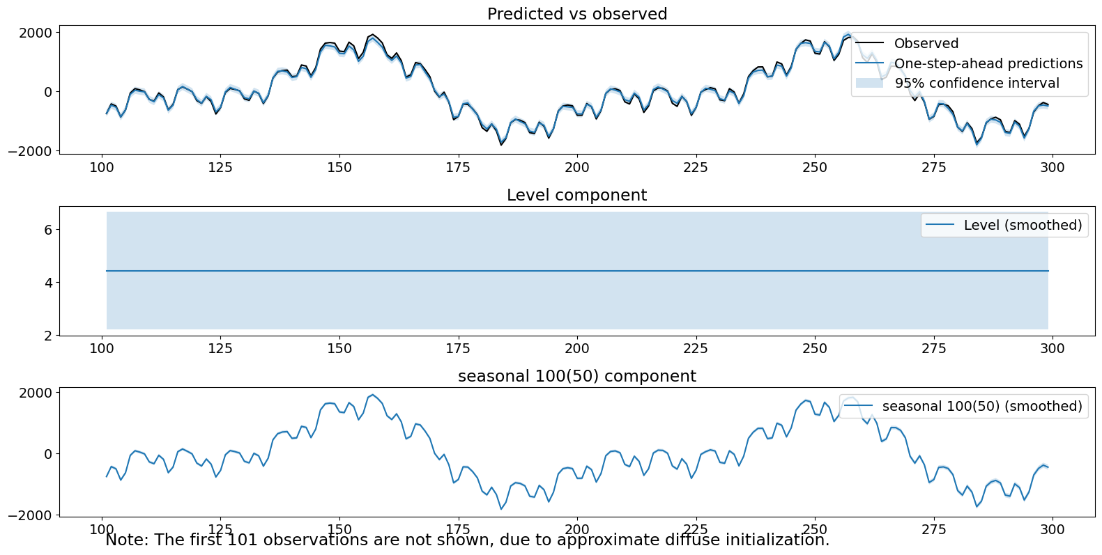
請注意,我們的診斷檢定之一將在 .05 水準上被拒絕。
未觀測到的成分 (惰性時域季節性建模)
第四種方法是一個具有固定截距和一個使用 100 個常數的時域季節性模型建模的單一季節性成分的未觀測到的成分模型。時間序列的過程可以寫成
其中 \(\epsilon_t\) 是白雜訊,\(\omega^{(1)}_{t}\) 是獨立同分布的 \(N(0, \sigma^2_1)\)。
[9]:
model = sm.tsa.UnobservedComponents(series,
                                    level='fixed intercept',
                                    seasonal=100)
res_lt = model.fit(disp=False)
print(res_lt.summary())
# The first state variable holds our estimate of the intercept
print("fixed intercept estimated as {0:.3f}".format(res_lt.smoother_results.smoothed_state[0,-1:][0]))

fig = res_lt.plot_components()
fig.tight_layout(pad=1.0)
                            Unobserved Components Results
======================================================================================
Dep. Variable:                              y   No. Observations:                  300
Model:                        fixed intercept   Log Likelihood               -1564.378
                   + stochastic seasonal(100)   AIC                           3130.756
Date:                        Thu, 03 Oct 2024   BIC                           3134.054
Time:                                16:07:26   HQIC                          3132.091
Sample:                                     0
                                        - 300
Covariance Type:                          opg
===================================================================================
                      coef    std err          z      P>|z|      [0.025      0.975]
-----------------------------------------------------------------------------------
sigma2.seasonal  3.558e+05   2.96e+04     12.012      0.000    2.98e+05    4.14e+05
===================================================================================
Ljung-Box (L1) (Q):                 200.79   Jarque-Bera (JB):                25.29
Prob(Q):                              0.00   Prob(JB):                         0.00
Heteroskedasticity (H):               0.49   Skew:                             0.85
Prob(H) (two-sided):                  0.00   Kurtosis:                         3.37
===================================================================================

Warnings:
[1] Covariance matrix calculated using the outer product of gradients (complex-step).
fixed intercept estimated as 4.690
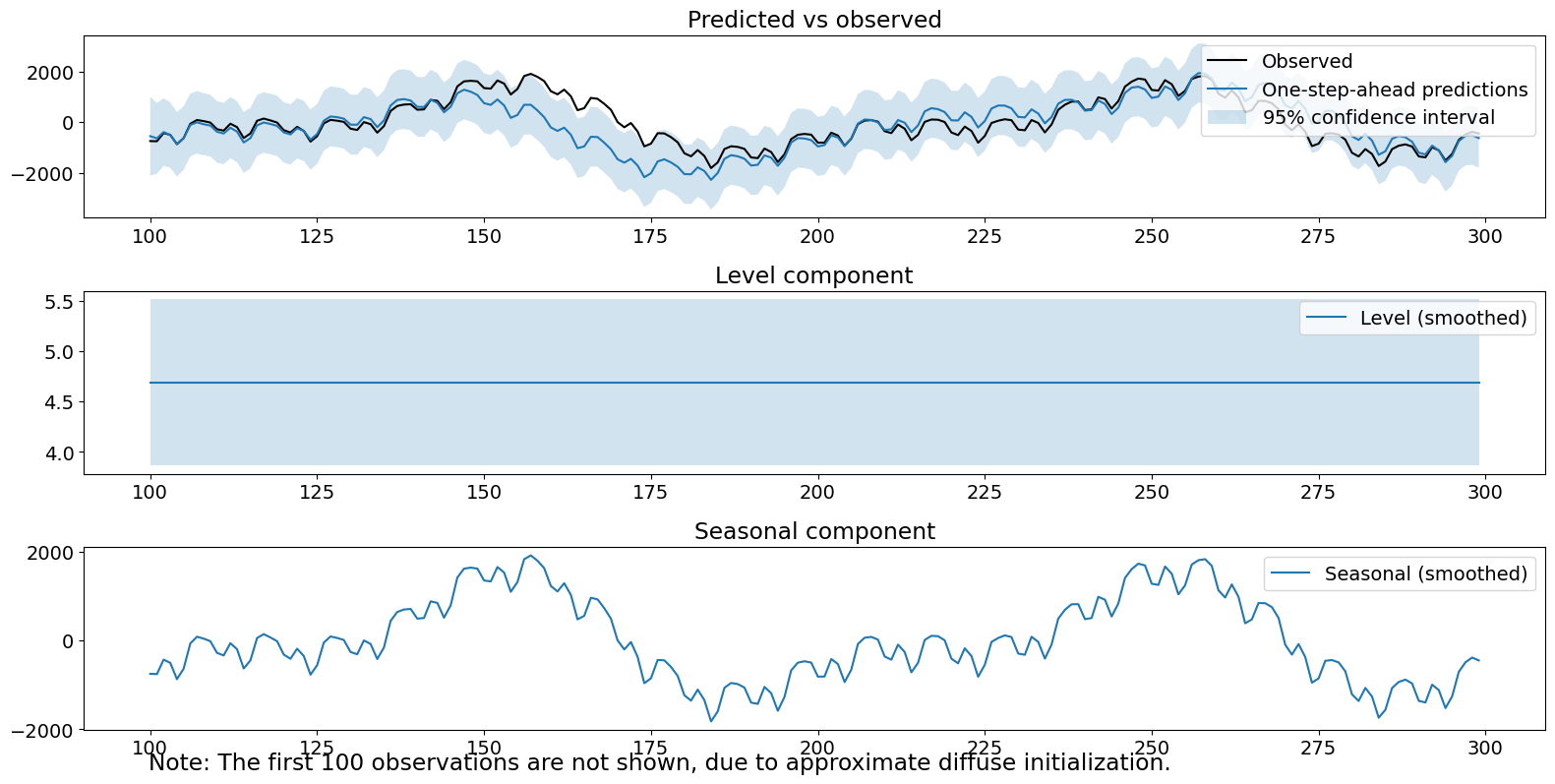
季節性成分本身看起來不錯——它是主要訊號。季節性項的估計變異數非常高 (\(>10^5\)),導致我們單步向前預測中存在大量的不確定性,並且對新資料的反應緩慢,從單步向前預測和觀測中的巨大誤差可以看出。最後,我們所有三項診斷檢定都被拒絕了。
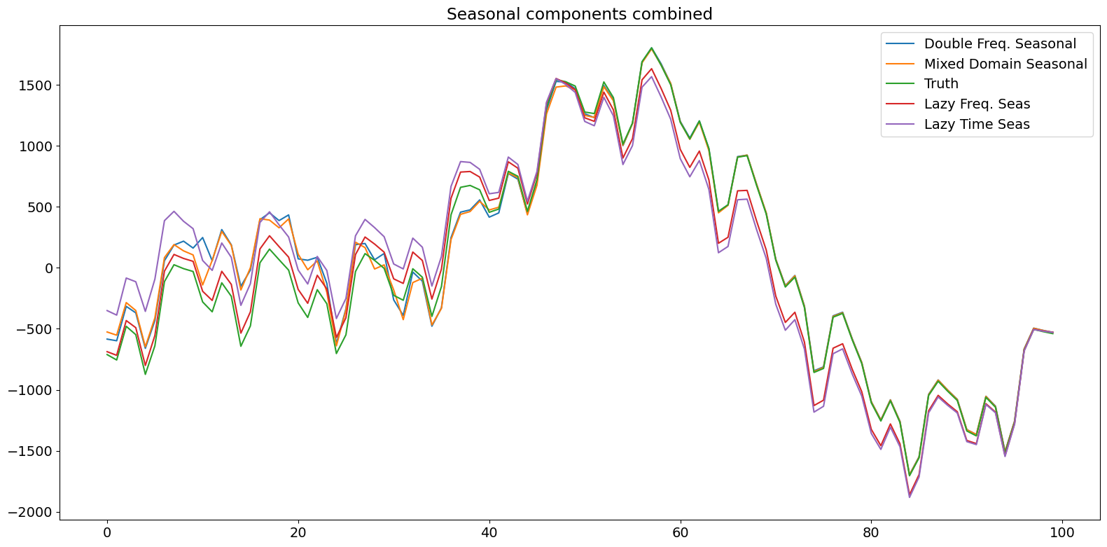
過濾估計值的比較
下面的圖表顯示,明確地對各個成分進行建模會導致過濾後的狀態在約一半週期內接近真實狀態。惰性模型需要更長的時間 (幾乎是一個完整的週期) 才能在組合的真實狀態上執行相同的操作。
[10]:
# Assign better names for our seasonal terms
true_seasonal_10_3 = terms[0]
true_seasonal_100_2 = terms[1]
true_sum = true_seasonal_10_3 + true_seasonal_100_2
[11]:
time_s = np.s_[:50]  # After this they basically agree
fig1 = plt.figure()
ax1 = fig1.add_subplot(111)
idx = np.asarray(series.index)
h1, = ax1.plot(idx[time_s], res_f.freq_seasonal[0].filtered[time_s], label='Double Freq. Seas')
h2, = ax1.plot(idx[time_s], res_tf.seasonal.filtered[time_s], label='Mixed Domain Seas')
h3, = ax1.plot(idx[time_s], true_seasonal_10_3[time_s], label='True Seasonal 10(3)')
plt.legend([h1, h2, h3], ['Double Freq. Seasonal','Mixed Domain Seasonal','Truth'], loc=2)
plt.title('Seasonal 10(3) component')
plt.show()
[12]:
time_s = np.s_[:50]  # After this they basically agree
fig2 = plt.figure()
ax2 = fig2.add_subplot(111)
h21, = ax2.plot(idx[time_s], res_f.freq_seasonal[1].filtered[time_s], label='Double Freq. Seas')
h22, = ax2.plot(idx[time_s], res_tf.freq_seasonal[0].filtered[time_s], label='Mixed Domain Seas')
h23, = ax2.plot(idx[time_s], true_seasonal_100_2[time_s], label='True Seasonal 100(2)')
plt.legend([h21, h22, h23], ['Double Freq. Seasonal','Mixed Domain Seasonal','Truth'], loc=2)
plt.title('Seasonal 100(2) component')
plt.show()
[13]:
time_s = np.s_[:100]

fig3 = plt.figure()
ax3 = fig3.add_subplot(111)
h31, = ax3.plot(idx[time_s], res_f.freq_seasonal[1].filtered[time_s] + res_f.freq_seasonal[0].filtered[time_s], label='Double Freq. Seas')
h32, = ax3.plot(idx[time_s], res_tf.freq_seasonal[0].filtered[time_s] + res_tf.seasonal.filtered[time_s], label='Mixed Domain Seas')
h33, = ax3.plot(idx[time_s], true_sum[time_s], label='True Seasonal 100(2)')
h34, = ax3.plot(idx[time_s], res_lf.freq_seasonal[0].filtered[time_s], label='Lazy Freq. Seas')
h35, = ax3.plot(idx[time_s], res_lt.seasonal.filtered[time_s], label='Lazy Time Seas')

plt.legend([h31, h32, h33, h34, h35], ['Double Freq. Seasonal','Mixed Domain Seasonal','Truth', 'Lazy Freq. Seas', 'Lazy Time Seas'], loc=1)
plt.title('Seasonal components combined')
plt.tight_layout(pad=1.0)
結論
在本筆記本中,我們模擬了一個具有兩個不同週期季節性成分的時間序列。我們使用結構時間序列模型對其進行建模,其中 (a) 兩個具有正確週期和諧波數的頻域成分,(b) 短期時間域季節性成分和具有正確週期和諧波數的頻域項,(c) 單個具有較長週期和完整諧波數的頻域項,以及 (d) 單個具有較長週期的時間域項。我們看到了各種診斷結果,其中只有正確的生成模型 (a) 未能拒絕任何測試。因此,更靈活的季節性建模,允許使用具有可指定諧波的多個成分,可以成為時間序列建模的有用工具。最後,我們可以通過這種方式用更少的總狀態來表示季節性成分,允許用戶嘗試自己進行偏差-變異權衡,而不是被迫選擇使用大量狀態並因此產生額外變異的「惰性」模型。