SARIMAX:簡介
這個筆記本重現了來自 Stata ARIMA 時間序列估計和後估計文件的範例。
首先,我們重現四個估計範例 http://www.stata.com/manuals13/tsarima.pdf
美國批發物價指數 (WPI) 資料集上的 ARIMA(1,1,1) 模型。
範例 1 的變體,它將 MA(4) 項添加到 ARIMA(1,1,1) 規範中,以允許加法季節效應。
每月航空公司資料的 ARIMA(2,1,0) x (1,1,0,12) 模型。這個範例允許乘法季節效應。
具有外生迴歸變數的 ARMA(1,1) 模型;將消費描述為一個自迴歸過程,其中也假設貨幣供應量是一個解釋變數。
其次,我們展示了後估計能力以重現 http://www.stata.com/manuals13/tsarimapostestimation.pdf。範例 4 中的模型用於示範
一步提前的樣本內預測
n 步提前的樣本外預測
n 步提前的樣本內動態預測
[1]:
%matplotlib inline
[2]:
import numpy as np
import pandas as pd
from scipy.stats import norm
import statsmodels.api as sm
import matplotlib.pyplot as plt
from datetime import datetime
import requests
from io import BytesIO
# Register converters to avoid warnings
pd.plotting.register_matplotlib_converters()
plt.rc("figure", figsize=(16,8))
plt.rc("font", size=14)
ARIMA 範例 1:Arima
正如範例 2 中的圖表所見,批發物價指數 (WPI) 隨著時間的推移而增長(即不是平穩的)。因此,ARMA 模型不是一個好的規範。在這個第一個範例中,我們考慮一個模型,其中假設原始時間序列的積分階數為 1,因此假設差異是平穩的,並且擬合一個具有一個自迴歸滯後和一個移動平均滯後的模型,以及一個截距項。
然後假設的資料過程是
其中 \(c\) 是 ARMA 模型的截距,\(\Delta\) 是第一差分運算子,並且我們假設 \(\epsilon_{t} \sim N(0, \sigma^2)\)。這可以重寫以強調滯後多項式(這在下面的範例 2 中很有用)
其中 \(L\) 是滯後運算子。
請注意,Stata 輸出和下面的輸出之間的一個區別是,Stata 估計了以下模型
其中 \(\beta_0\) 是過程 \(y_t\) 的平均值。此模型等效於 statsmodels SARIMAX 類中估計的模型,但解釋不同。為了看到等效性,請注意
因此 \(c = (1 - \phi_1) \beta_0\)。
[3]:
# Dataset
wpi1 = requests.get('https://www.stata-press.com/data/r12/wpi1.dta').content
data = pd.read_stata(BytesIO(wpi1))
data.index = data.t
# Set the frequency
data.index.freq="QS-OCT"

# Fit the model
mod = sm.tsa.statespace.SARIMAX(data['wpi'], trend='c', order=(1,1,1))
res = mod.fit(disp=False)
print(res.summary())
                               SARIMAX Results
==============================================================================
Dep. Variable:                    wpi   No. Observations:                  124
Model:               SARIMAX(1, 1, 1)   Log Likelihood                -135.351
Date:                Thu, 03 Oct 2024   AIC                            278.703
Time:                        16:05:55   BIC                            289.951
Sample:                    01-01-1960   HQIC                           283.272
                         - 10-01-1990
Covariance Type:                  opg
==============================================================================
                 coef    std err          z      P>|z|      [0.025      0.975]
------------------------------------------------------------------------------
intercept      0.0943      0.068      1.389      0.165      -0.039       0.227
ar.L1          0.8742      0.055     16.028      0.000       0.767       0.981
ma.L1         -0.4120      0.100     -4.119      0.000      -0.608      -0.216
sigma2         0.5257      0.053      9.849      0.000       0.421       0.630
===================================================================================
Ljung-Box (L1) (Q):                   0.09   Jarque-Bera (JB):                 9.78
Prob(Q):                              0.77   Prob(JB):                         0.01
Heteroskedasticity (H):              15.93   Skew:                             0.28
Prob(H) (two-sided):                  0.00   Kurtosis:                         4.26
===================================================================================

Warnings:
[1] Covariance matrix calculated using the outer product of gradients (complex-step).
因此,最大概似估計意味著對於上面的過程,我們有
其中 \(\epsilon_{t} \sim N(0, 0.5257)\)。最後,回想一下 \(c = (1 - \phi_1) \beta_0\),這裡 \(c = 0.0943\) 且 \(\phi_1 = 0.8742\)。為了與 Stata 的輸出進行比較,我們可以計算平均值
注意:此值與 Stata 文件中的值 \(\beta_0 = 0.7498\) 幾乎相同。細微的差異可能歸因於四捨五入和所用數值優化器的停止準則的細微差異。
ARIMA 範例 2:具有加法季節效應的 Arima
此模型是範例 1 的延伸。這裡假設資料遵循該過程
這個模型的新部分是允許有年度季節效應(即使週期是 4,因為資料集是季度的)。第二個不同之處在於此模型使用資料的對數而不是水平值。
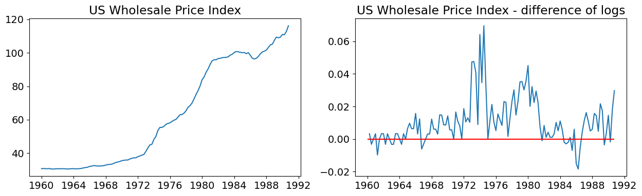
在估計資料集之前,圖表顯示
時間序列(以對數表示)
時間序列的第一差分(以對數表示)
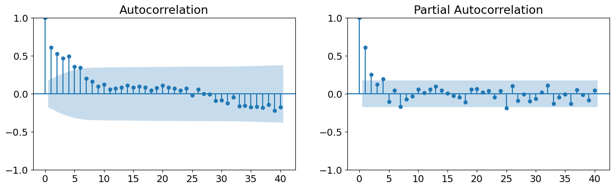
自相關函數
偏自相關函數。
從前兩個圖表中,我們注意到原始時間序列似乎不是平穩的,而第一差分是平穩的。這支持在資料的第一差分上估計 ARMA 模型,或者估計具有 1 個積分階數的 ARIMA 模型(回想一下我們正在採用後者的方法)。最後兩個圖表支持使用 ARMA(1,1,1) 模型。
[4]:
# Dataset
data = pd.read_stata(BytesIO(wpi1))
data.index = data.t
data.index.freq="QS-OCT"

data['ln_wpi'] = np.log(data['wpi'])
data['D.ln_wpi'] = data['ln_wpi'].diff()
[5]:
# Graph data
fig, axes = plt.subplots(1, 2, figsize=(15,4))

# Levels
axes[0].plot(data.index._mpl_repr(), data['wpi'], '-')
axes[0].set(title='US Wholesale Price Index')

# Log difference
axes[1].plot(data.index._mpl_repr(), data['D.ln_wpi'], '-')
axes[1].hlines(0, data.index[0], data.index[-1], 'r')
axes[1].set(title='US Wholesale Price Index - difference of logs');
[6]:
# Graph data
fig, axes = plt.subplots(1, 2, figsize=(15,4))

fig = sm.graphics.tsa.plot_acf(data.iloc[1:]['D.ln_wpi'], lags=40, ax=axes[0])
fig = sm.graphics.tsa.plot_pacf(data.iloc[1:]['D.ln_wpi'], lags=40, ax=axes[1])
為了了解如何在 statsmodels 中指定此模型,首先回想一下,在範例 1 中,我們使用了以下程式碼來指定 ARIMA(1,1,1) 模型
mod = sm.tsa.statespace.SARIMAX(data['wpi'], trend='c', order=(1,1,1))
order 引數是形式為 (AR 規範、 積分 階數、 MA 規範) 的元組。積分階數必須是整數(例如,這裡我們假設一個積分階數,因此指定為 1。在底層資料已經平穩的純 ARMA 模型中,它將為 0)。
對於 AR 規範和 MA 規範元件,有兩種可能性。第一種是指定對應滯後多項式的最大度數,在這種情況下,元件是一個整數。例如,如果我們想指定 ARIMA(1,1,4) 過程,我們將使用
mod = sm.tsa.statespace.SARIMAX(data['wpi'], trend='c', order=(1,1,4))
對應的資料過程將是
或
當規範參數給定為滯後多項式的最大度數時,這表示包括直到該度數的所有多項式項。請注意,這不是我們要使用的模型,因為它將包括 \(\epsilon_{t-2}\) 和 \(\epsilon_{t-3}\) 的項,而我們在這裡不需要這些項。
我們想要的是一個具有第 1 和第 4 度項,但省略第 2 和第 3 項的多項式。為此,我們需要為規範參數提供一個元組,其中元組描述了滯後多項式本身。特別是,在這裡我們想使用
ar = 1          # this is the maximum degree specification
ma = (1,0,0,1)  # this is the lag polynomial specification
mod = sm.tsa.statespace.SARIMAX(data['wpi'], trend='c', order=(ar,1,ma)))
這給出了資料過程的以下形式
這正是我們想要的。
[7]:
# Fit the model
mod = sm.tsa.statespace.SARIMAX(data['ln_wpi'], trend='c', order=(1,1,(1,0,0,1)))
res = mod.fit(disp=False)
print(res.summary())
                                 SARIMAX Results
=================================================================================
Dep. Variable:                    ln_wpi   No. Observations:                  124
Model:             SARIMAX(1, 1, [1, 4])   Log Likelihood                 386.034
Date:                   Thu, 03 Oct 2024   AIC                           -762.067
Time:                           16:06:14   BIC                           -748.006
Sample:                       01-01-1960   HQIC                          -756.355
                            - 10-01-1990
Covariance Type:                     opg
==============================================================================
                 coef    std err          z      P>|z|      [0.025      0.975]
------------------------------------------------------------------------------
intercept      0.0024      0.002      1.485      0.138      -0.001       0.006
ar.L1          0.7808      0.094      8.269      0.000       0.596       0.966
ma.L1         -0.3993      0.126     -3.174      0.002      -0.646      -0.153
ma.L4          0.3087      0.120      2.572      0.010       0.073       0.544
sigma2         0.0001    9.8e-06     11.114      0.000    8.97e-05       0.000
===================================================================================
Ljung-Box (L1) (Q):                   0.02   Jarque-Bera (JB):                45.15
Prob(Q):                              0.90   Prob(JB):                         0.00
Heteroskedasticity (H):               2.58   Skew:                             0.29
Prob(H) (two-sided):                  0.00   Kurtosis:                         5.91
===================================================================================

Warnings:
[1] Covariance matrix calculated using the outer product of gradients (complex-step).
ARIMA 範例 3:航空公司模型
在上一個範例中,我們以加法方式包含季節效應,這意味著我們添加一個項,允許該過程取決於第 4 個 MA 滯後。我們可能反而希望以乘法方式對季節效應建模。我們通常將模型寫為 ARIMA \((p,d,q) \times (P,D,Q)_s\),其中小寫字母表示非季節性成分的規範,大寫字母表示季節性成分的規範;\(s\) 是季節的週期性(例如,季度資料通常為 4,每月資料通常為 12)。資料過程可以泛化地寫為
其中
\(\phi_p (L)\) 是非季節自迴歸滯後多項式
\(\tilde \phi_P (L^s)\) 是季節性自迴歸滯後多項式
\(\Delta^d \Delta_s^D y_t\) 是時間序列,已差分 \(d\) 次,並且已季節性差分 \(D\) 次。
\(A(t)\) 是趨勢多項式(包括截距)
\(\theta_q (L)\) 是非季節性移動平均滯後多項式
\(\tilde \theta_Q (L^s)\) 是季節性移動平均滯後多項式
有時我們將其重寫為
其中 \(y_t^* = \Delta^d \Delta_s^D y_t\)。這強調了如同簡單情況,在我們進行差分(此處包含非季節性和季節性差分)使數據平穩後,得到的模型只是一個 ARMA 模型。
舉例來說,考慮包含截距的航空模型 ARIMA \((2,1,0) \times (1,1,0)_{12}\)。數據過程可以寫成上述形式:
在這裡,我們有
\(\phi_p (L) = (1 - \phi_1 L - \phi_2 L^2)\)
\(\tilde \phi_P (L^s) = (1 - \phi_1 L^{12})\)
\(d = 1, D = 1, s=12\),表示 \(y_t^*\) 是由 \(y_t\) 經由一次差分,然後再經過 12 次差分得到的。
\(A(t) = c\) 是一個常數趨勢多項式(即僅為一個截距)。
\(\theta_q (L) = \tilde \theta_Q (L^s) = 1\)(即沒有移動平均效應)。
看到時間序列變數前有兩個滯後多項式可能會感到困惑,但請注意,我們可以將這些滯後多項式相乘得到以下模型:
這可以改寫為:
這類似於範例 2 中的加法季節性模型,但自迴歸滯後的係數實際上是基礎季節性和非季節性參數的組合。
在 statsmodels 中指定模型只需添加 seasonal_order 參數,該參數接受形式為 (季節性 AR 規格、季節性整合階數、季節性 MA、季節性週期) 的元組。與之前一樣,季節性 AR 和 MA 規格可以用最大多項式次數或滯後多項式本身表示。季節性週期是一個整數。
對於包含截距的航空模型 ARIMA \((2,1,0) \times (1,1,0)_{12}\),指令如下:
mod = sm.tsa.statespace.SARIMAX(data['lnair'], order=(2,1,0), seasonal_order=(1,1,0,12))
[8]:
# Dataset
air2 = requests.get('https://www.stata-press.com/data/r12/air2.dta').content
data = pd.read_stata(BytesIO(air2))
data.index = pd.date_range(start=datetime(int(data.time[0]), 1, 1), periods=len(data), freq='MS')
data['lnair'] = np.log(data['air'])

# Fit the model
mod = sm.tsa.statespace.SARIMAX(data['lnair'], order=(2,1,0), seasonal_order=(1,1,0,12), simple_differencing=True)
res = mod.fit(disp=False)
print(res.summary())
                                     SARIMAX Results
==========================================================================================
Dep. Variable:                       D.DS12.lnair   No. Observations:                  131
Model:             SARIMAX(2, 0, 0)x(1, 0, 0, 12)   Log Likelihood                 240.821
Date:                            Thu, 03 Oct 2024   AIC                           -473.643
Time:                                    16:06:19   BIC                           -462.142
Sample:                                02-01-1950   HQIC                          -468.970
                                     - 12-01-1960
Covariance Type:                              opg
==============================================================================
                 coef    std err          z      P>|z|      [0.025      0.975]
------------------------------------------------------------------------------
ar.L1         -0.4057      0.080     -5.045      0.000      -0.563      -0.248
ar.L2         -0.0799      0.099     -0.809      0.419      -0.274       0.114
ar.S.L12      -0.4723      0.072     -6.592      0.000      -0.613      -0.332
sigma2         0.0014      0.000      8.403      0.000       0.001       0.002
===================================================================================
Ljung-Box (L1) (Q):                   0.01   Jarque-Bera (JB):                 0.72
Prob(Q):                              0.91   Prob(JB):                         0.70
Heteroskedasticity (H):               0.54   Skew:                             0.14
Prob(H) (two-sided):                  0.04   Kurtosis:                         3.23
===================================================================================

Warnings:
[1] Covariance matrix calculated using the outer product of gradients (complex-step).
請注意,這裡我們使用了一個額外的參數 simple_differencing=True。這控制著 ARIMA 模型中如何處理整合階數。如果 simple_differencing=True,則作為 endog 提供的時間序列會被直接差分,並且將 ARMA 模型擬合到產生的新時間序列。這意味著一些初始週期會在差分過程中遺失,但這可能是為了與其他套件的結果(例如,Stata 的 arima 始終使用簡單差分)進行比較,或者當季節性週期很大時所必需的。
預設值為 simple_differencing=False,在這種情況下,整合組件會作為狀態空間公式的一部分來實現,並且所有原始數據都可以在估計中使用。
ARIMA 範例 4:ARMAX(Friedman)
此模型示範了解釋變數(ARMAX 的 X 部分)的使用。當包含外生迴歸因子時,SARIMAX 模組使用「具有 SARIMA 誤差的迴歸」的概念(有關具有 ARIMA 誤差的迴歸與其他規格的詳細資訊,請參閱 http://robjhyndman.com/hyndsight/arimax/),因此模型被指定為:
請注意,第一個方程式只是一個線性迴歸,而第二個方程式只描述了誤差組件遵循 SARIMA 的過程(如範例 3 中所述)。此規格的原因之一是估計的參數具有其自然的解釋。
此規格嵌套了許多更簡單的規格。例如,具有 AR(2) 誤差的迴歸為:
此範例中考慮的模型是具有 ARMA(1,1) 誤差的迴歸。然後,該過程被寫為:
請注意,如上述範例 1 中所述,\(\beta_0\) 與由 trend='c' 指定的截距不同。雖然在上面的範例中,我們透過趨勢多項式來估計模型的截距,但在這裡,我們示範如何透過將常數添加到外生數據集來估計 \(\beta_0\) 本身。在輸出中,\(beta_0\) 被稱為 const,而上面的截距 \(c\) 在輸出中被稱為 intercept。
[9]:
# Dataset
friedman2 = requests.get('https://www.stata-press.com/data/r12/friedman2.dta').content
data = pd.read_stata(BytesIO(friedman2))
data.index = data.time
data.index.freq = "QS-OCT"

# Variables
endog = data.loc['1959':'1981', 'consump']
exog = sm.add_constant(data.loc['1959':'1981', 'm2'])

# Fit the model
mod = sm.tsa.statespace.SARIMAX(endog, exog, order=(1,0,1))
res = mod.fit(disp=False)
print(res.summary())
                               SARIMAX Results
==============================================================================
Dep. Variable:                consump   No. Observations:                   92
Model:               SARIMAX(1, 0, 1)   Log Likelihood                -340.508
Date:                Thu, 03 Oct 2024   AIC                            691.015
Time:                        16:06:21   BIC                            703.624
Sample:                    01-01-1959   HQIC                           696.105
                         - 10-01-1981
Covariance Type:                  opg
==============================================================================
                 coef    std err          z      P>|z|      [0.025      0.975]
------------------------------------------------------------------------------
const        -36.0606     56.643     -0.637      0.524    -147.078      74.957
m2             1.1220      0.036     30.824      0.000       1.051       1.193
ar.L1          0.9348      0.041     22.717      0.000       0.854       1.015
ma.L1          0.3091      0.089      3.488      0.000       0.135       0.483
sigma2        93.2556     10.889      8.565      0.000      71.914     114.597
===================================================================================
Ljung-Box (L1) (Q):                   0.04   Jarque-Bera (JB):                23.49
Prob(Q):                              0.84   Prob(JB):                         0.00
Heteroskedasticity (H):              22.51   Skew:                             0.17
Prob(H) (two-sided):                  0.00   Kurtosis:                         5.45
===================================================================================

Warnings:
[1] Covariance matrix calculated using the outer product of gradients (complex-step).
ARIMA 後估計:範例 1 - 動態預測
在這裡,我們描述 statsmodels 的 SARIMAX 的一些後估計功能。
首先,使用範例中的模型,我們使用排除最後幾個觀察值的數據來估計參數(作為範例這有點人工,但它允許考慮樣本外預測的效能,並方便與 Stata 的文件進行比較)。
[10]:
# Dataset
raw = pd.read_stata(BytesIO(friedman2))
raw.index = raw.time
raw.index.freq = "QS-OCT"
data = raw.loc[:'1981']

# Variables
endog = data.loc['1959':, 'consump']
exog = sm.add_constant(data.loc['1959':, 'm2'])
nobs = endog.shape[0]

# Fit the model
mod = sm.tsa.statespace.SARIMAX(endog.loc[:'1978-01-01'], exog=exog.loc[:'1978-01-01'], order=(1,0,1))
fit_res = mod.fit(disp=False, maxiter=250)
print(fit_res.summary())
                               SARIMAX Results
==============================================================================
Dep. Variable:                consump   No. Observations:                   77
Model:               SARIMAX(1, 0, 1)   Log Likelihood                -243.316
Date:                Thu, 03 Oct 2024   AIC                            496.633
Time:                        16:06:22   BIC                            508.352
Sample:                    01-01-1959   HQIC                           501.320
                         - 01-01-1978
Covariance Type:                  opg
==============================================================================
                 coef    std err          z      P>|z|      [0.025      0.975]
------------------------------------------------------------------------------
const          0.6782     18.492      0.037      0.971     -35.565      36.922
m2             1.0379      0.021     50.329      0.000       0.997       1.078
ar.L1          0.8775      0.059     14.859      0.000       0.762       0.993
ma.L1          0.2771      0.108      2.572      0.010       0.066       0.488
sigma2        31.6979      4.683      6.769      0.000      22.520      40.876
===================================================================================
Ljung-Box (L1) (Q):                   0.32   Jarque-Bera (JB):                 6.05
Prob(Q):                              0.57   Prob(JB):                         0.05
Heteroskedasticity (H):               6.09   Skew:                             0.57
Prob(H) (two-sided):                  0.00   Kurtosis:                         3.76
===================================================================================

Warnings:
[1] Covariance matrix calculated using the outer product of gradients (complex-step).
接下來,我們想要獲得完整數據集的結果,但使用估計的參數(在數據的子集上)。
[11]:
mod = sm.tsa.statespace.SARIMAX(endog, exog=exog, order=(1,0,1))
res = mod.filter(fit_res.params)
predict 命令首先在此處應用以獲得樣本內預測。我們使用 full_results=True 參數來允許我們計算信賴區間(predict 的預設輸出僅為預測值)。
在沒有其他參數的情況下,predict 會針對整個樣本傳回單步提前的樣本內預測。
[12]:
# In-sample one-step-ahead predictions
predict = res.get_prediction()
predict_ci = predict.conf_int()
我們也可以獲得動態預測。單步提前預測使用每個步驟的內生變數的真實值來預測下一個樣本內值。動態預測在數據集中使用單步提前預測直到某個點(由 dynamic 參數指定);之後,先前預測的內生值將被用來代替每個新預測元素的真實內生值。
dynamic 參數被指定為相對於 start 參數的偏移量。如果未指定 start,則假定其為 0。
在這裡,我們執行從 1978 年第一季開始的動態預測。
[13]:
# Dynamic predictions
predict_dy = res.get_prediction(dynamic='1978-01-01')
predict_dy_ci = predict_dy.conf_int()
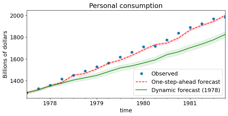
我們可以繪製單步提前和動態預測(以及相應的信賴區間)的圖形,以查看它們的相對效能。請注意,直到動態預測開始的點(1978 年第一季),兩者是相同的。
[14]:
# Graph
fig, ax = plt.subplots(figsize=(9,4))
npre = 4
ax.set(title='Personal consumption', xlabel='Date', ylabel='Billions of dollars')

# Plot data points
data.loc['1977-07-01':, 'consump'].plot(ax=ax, style='o', label='Observed')

# Plot predictions
predict.predicted_mean.loc['1977-07-01':].plot(ax=ax, style='r--', label='One-step-ahead forecast')
ci = predict_ci.loc['1977-07-01':]
ax.fill_between(ci.index, ci.iloc[:,0], ci.iloc[:,1], color='r', alpha=0.1)
predict_dy.predicted_mean.loc['1977-07-01':].plot(ax=ax, style='g', label='Dynamic forecast (1978)')
ci = predict_dy_ci.loc['1977-07-01':]
ax.fill_between(ci.index, ci.iloc[:,0], ci.iloc[:,1], color='g', alpha=0.1)

legend = ax.legend(loc='lower right')
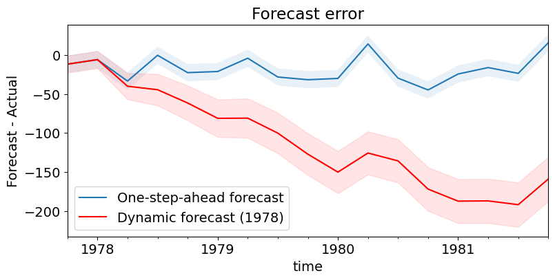
最後,繪製預測誤差的圖形。很明顯,正如人們所懷疑的那樣,單步提前預測顯然要好得多。
[15]:
# Prediction error

# Graph
fig, ax = plt.subplots(figsize=(9,4))
npre = 4
ax.set(title='Forecast error', xlabel='Date', ylabel='Forecast - Actual')

# In-sample one-step-ahead predictions and 95% confidence intervals
predict_error = predict.predicted_mean - endog
predict_error.loc['1977-10-01':].plot(ax=ax, label='One-step-ahead forecast')
ci = predict_ci.loc['1977-10-01':].copy()
ci.iloc[:,0] -= endog.loc['1977-10-01':]
ci.iloc[:,1] -= endog.loc['1977-10-01':]
ax.fill_between(ci.index, ci.iloc[:,0], ci.iloc[:,1], alpha=0.1)

# Dynamic predictions and 95% confidence intervals
predict_dy_error = predict_dy.predicted_mean - endog
predict_dy_error.loc['1977-10-01':].plot(ax=ax, style='r', label='Dynamic forecast (1978)')
ci = predict_dy_ci.loc['1977-10-01':].copy()
ci.iloc[:,0] -= endog.loc['1977-10-01':]
ci.iloc[:,1] -= endog.loc['1977-10-01':]
ax.fill_between(ci.index, ci.iloc[:,0], ci.iloc[:,1], color='r', alpha=0.1)

legend = ax.legend(loc='lower left');
legend.get_frame().set_facecolor('w')