預測、更新資料集和「消息」
在本筆記本中,我們描述如何使用 Statsmodels 來計算更新或修訂的資料集對樣本外預測或遺失資料的樣本內估計的影響。我們遵循「即時預測」文獻(請參閱文末的參考文獻)的方法,使用狀態空間模型來計算傳入資料的「消息」和影響。
注意:此筆記本適用於 Statsmodels v0.12+。此外,它僅適用於狀態空間模型或相關類別,包括:sm.tsa.statespace.ExponentialSmoothing、sm.tsa.arima.ARIMA、sm.tsa.SARIMAX、sm.tsa.UnobservedComponents、sm.tsa.VARMAX 和 sm.tsa.DynamicFactor。
[1]:
%matplotlib inline

import numpy as np
import pandas as pd
import statsmodels.api as sm
import matplotlib.pyplot as plt

macrodata = sm.datasets.macrodata.load_pandas().data
macrodata.index = pd.period_range('1959Q1', '2009Q3', freq='Q')
預測練習通常從一組固定的歷史資料開始,這些資料用於模型選擇和參數估計。然後,可以使用擬合的選定模型(或多個模型)來建立樣本外預測。大多數時候,這不是故事的結局。隨著新資料的到來,您可能需要評估您的預測誤差,可能更新您的模型,並建立更新的樣本外預測。這有時稱為「即時」預測練習(相比之下,偽即時練習是模擬此程序的一種)。
如果所有重要的是最小化基於預測誤差的某些損失函數(如 MSE),那麼當新資料出現時,您可能只想使用更新的資料點完全重新執行模型選擇、參數估計和樣本外預測。如果您這樣做,您的新預測將因兩個原因而改變
您已收到提供新資訊的新資料
您的預測模型或估計的參數不同
在本筆記本中,我們專注於隔離第一種效果的方法。我們這樣做的方式來自所謂的「即時預測」文獻,特別是 Bańbura、Giannone 和 Reichlin (2011)、Bańbura 和 Modugno (2014) 以及 Bańbura 等人 (2014)。他們將此練習描述為計算「消息」,我們遵循他們在 Statsmodels 中使用這種語言。
這些方法可能在多變數模型中最有用,因為多個變數可能會同時更新,並且哪些更新的變數導致了哪些預測變化並不立即顯而易見。但是,它們仍然可以用於考慮單變數模型中的預測修訂。因此,我們將從較簡單的單變數案例開始,解釋其工作原理,然後再轉到多變數案例。
關於修訂的注意事項:我們正在使用的框架旨在分解來自新觀測到的資料點的預測變更。它還可以考慮對先前發布的資料點的修訂,但它不會單獨分解它們。相反,它僅顯示「修訂」的總體效果。
關於 ``exog`` 資料的注意事項:我們正在使用的框架僅分解來自針對建模變數的新觀測資料點的預測變更。這些是 Statsmodels 中在 endog 參數中給出的「左側」變數。此框架不會分解或考慮未建模的「右側」變數的變更,例如包含在 exog 參數中的那些變數。
簡單的單變數範例:AR(1)
我們將從一個簡單的自迴歸模型開始,即 AR(1)
參數 \(\phi\) 捕捉了序列的持續性
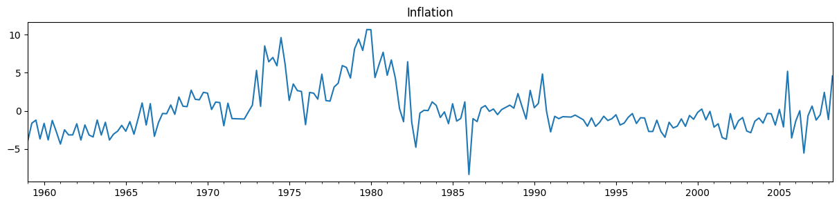
我們將使用此模型來預測通膨。
為了使在本筆記本中描述預測更新更容易,我們將使用已去平均值的通膨資料,但在實踐中,使用平均值項來增強模型是很簡單的。
[2]:
# De-mean the inflation series
y = macrodata['infl'] - macrodata['infl'].mean()
步驟 1:在可用的資料集上擬合模型
在這裡,我們將透過建構和擬合我們的模型,使用除了最後五個觀測值之外的所有資料來模擬一個樣本外練習。我們將假設我們尚未觀察到這些值,然後在後續步驟中,我們將它們新增回分析中。
[3]:
y_pre = y.iloc[:-5]
y_pre.plot(figsize=(15, 3), title='Inflation');
為了建構預測,我們首先估計模型的參數。這會傳回一個結果物件,我們可以使用該物件來產生預測。
[4]:
mod_pre = sm.tsa.arima.ARIMA(y_pre, order=(1, 0, 0), trend='n')
res_pre = mod_pre.fit()
print(res_pre.summary())
                               SARIMAX Results
==============================================================================
Dep. Variable:                   infl   No. Observations:                  198
Model:                 ARIMA(1, 0, 0)   Log Likelihood                -446.407
Date:                Thu, 03 Oct 2024   AIC                            896.813
Time:                        15:47:15   BIC                            903.390
Sample:                    03-31-1959   HQIC                           899.475
                         - 06-30-2008
Covariance Type:                  opg
==============================================================================
                 coef    std err          z      P>|z|      [0.025      0.975]
------------------------------------------------------------------------------
ar.L1          0.6751      0.043     15.858      0.000       0.592       0.759
sigma2         5.3027      0.367     14.459      0.000       4.584       6.022
===================================================================================
Ljung-Box (L1) (Q):                  15.65   Jarque-Bera (JB):                43.04
Prob(Q):                              0.00   Prob(JB):                         0.00
Heteroskedasticity (H):               0.85   Skew:                             0.18
Prob(H) (two-sided):                  0.50   Kurtosis:                         5.26
===================================================================================

Warnings:
[1] Covariance matrix calculated using the outer product of gradients (complex-step).
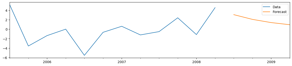
從結果物件 res 建立預測很容易 - 您只需使用要建構的預測數量呼叫 forecast 方法即可。在這種情況下,我們將建構四個樣本外預測。
[5]:
# Compute the forecasts
forecasts_pre = res_pre.forecast(4)

# Plot the last 3 years of data and the four out-of-sample forecasts
y_pre.iloc[-12:].plot(figsize=(15, 3), label='Data', legend=True)
forecasts_pre.plot(label='Forecast', legend=True);
對於 AR(1) 模型,手動建構預測也很容易。將最後觀測到的變數表示為 \(y_T\),將 \(h\) 步超前預測表示為 \(y_{T+h|T}\),我們有
其中 \(\hat \phi\) 是我們對 AR(1) 係數的估計值。從上面的摘要輸出中,我們可以知道這是模型的第一個參數,我們可以從結果物件的 params 屬性存取它。
[6]:
# Get the estimated AR(1) coefficient
phi_hat = res_pre.params[0]

# Get the last observed value of the variable
y_T = y_pre.iloc[-1]

# Directly compute the forecasts at the horizons h=1,2,3,4
manual_forecasts = pd.Series([phi_hat * y_T, phi_hat**2 * y_T,
                              phi_hat**3 * y_T, phi_hat**4 * y_T],
                             index=forecasts_pre.index)

# We'll print the two to double-check that they're the same
print(pd.concat([forecasts_pre, manual_forecasts], axis=1))
        predicted_mean         0
2008Q3        3.084388  3.084388
2008Q4        2.082323  2.082323
2009Q1        1.405812  1.405812
2009Q2        0.949088  0.949088
/tmp/ipykernel_4399/554023716.py:2: FutureWarning: Series.__getitem__ treating keys as positions is deprecated. In a future version, integer keys will always be treated as labels (consistent with DataFrame behavior). To access a value by position, use `ser.iloc[pos]`
  phi_hat = res_pre.params[0]
步驟 2:從新的觀測值計算「消息」
假設時間已經過去,我們現在收到另一個觀測值。我們的資料集現在更大,我們可以評估我們的預測誤差並產生後續季度的更新預測。
[7]:
# Get the next observation after the "pre" dataset
y_update = y.iloc[-5:-4]

# Print the forecast error
print('Forecast error: %.2f' % (y_update.iloc[0] - forecasts_pre.iloc[0]))
Forecast error: -10.21
為了基於我們更新的資料集計算預測,我們將使用 append 方法建立一個更新的結果物件 res_post,將我們的新觀測值附加到先前的資料集中。
請注意,預設情況下,append 方法不會重新估計模型的參數。這正是我們在這裡想要的,因為我們只想隔離新資訊對預測的影響。
[8]:
# Create a new results object by passing the new observations to the `append` method
res_post = res_pre.append(y_update)

# Since we now know the value for 2008Q3, we will only use `res_post` to
# produce forecasts for 2008Q4 through 2009Q2
forecasts_post = pd.concat([y_update, res_post.forecast('2009Q2')])
print(forecasts_post)
2008Q3   -7.121330
2008Q4   -4.807732
2009Q1   -3.245783
2009Q2   -2.191284
Freq: Q-DEC, dtype: float64
在這種情況下,預測誤差相當大 - 通膨比 AR(1) 模型的預測低了 10 個百分點以上。(這主要是因為全球金融危機前後的油價大幅波動)。
為了更深入地分析這一點,我們可以使用 Statsmodels 來隔離新資訊(或「消息」)對我們預測的影響。這表示我們還不想變更我們的模型或重新估計參數。相反,我們將使用狀態空間模型結果物件中提供的 news 方法。
在 Statsmodels 中計算消息始終需要先前的結果物件或資料集,以及更新的結果物件或資料集。在這裡,我們將使用原始結果物件 res_pre 作為先前的結果,並使用我們剛建立的 res_post 結果物件作為更新的結果。
一旦我們有了先前的和更新的結果物件或資料集,我們可以透過呼叫 news 方法來計算消息。在這裡,我們將呼叫 res_pre.news,第一個參數將是更新的結果 res_post(但是,如果您有兩個結果物件,則可以對其中一個呼叫 news 方法)。
除了將比較物件或資料集指定為第一個參數之外,還接受各種其他參數。最重要的參數指定您要考慮的「影響週期」。這些「影響週期」對應於感興趣的預測週期;也就是說,這些日期指定將分解哪些週期的預測修訂。
若要指定影響週期,您必須傳遞 start、end 和 periods 中的兩個(類似於 Pandas date_range 方法)。如果您的時間序列是具有關聯日期或週期索引的 Pandas 物件,則您可以傳遞日期作為 start 和 end 的值,如下所示。
[9]:
# Compute the impact of the news on the four periods that we previously
# forecasted: 2008Q3 through 2009Q2
news = res_pre.news(res_post, start='2008Q3', end='2009Q2')
# Note: one alternative way to specify these impact dates is
# `start='2008Q3', periods=4`
變數 news 是 NewsResults 類別的一個物件,其中包含關於與 res_pre 相比,res_post 中資料更新的詳細資訊、更新資料集中新的資訊,以及新資訊在 start 和 end 期間對預測的影響。
一個簡單總結結果的方法是使用 summary 方法。
[10]:
print(news.summary())
                                      News
===============================================================================
Model:                          ARIMA   Original sample:                 1959Q1
Date:                Thu, 03 Oct 2024                                  - 2008Q2
Time:                        15:47:16   Update through:                  2008Q3
                                        # of revisions:                       0
                                        # of new datapoints:                  1
          Impacts for [impacted variable = infl]
=========================================================
impact date estimate (prev) impact of news estimate (new)
---------------------------------------------------------
     2008Q3            3.08         -10.21          -7.12
     2008Q4            2.08          -6.89          -4.81
     2009Q1            1.41          -4.65          -3.25
     2009Q2            0.95          -3.14          -2.19
                  News from updated observations:
===================================================================
update date updated variable   observed forecast (prev)        news
-------------------------------------------------------------------
     2008Q3             infl      -7.12            3.08      -10.21
===================================================================
/opt/hostedtoolcache/Python/3.10.15/x64/lib/python3.10/site-packages/statsmodels/tsa/statespace/news.py:1328: FutureWarning: Setting an item of incompatible dtype is deprecated and will raise in a future error of pandas. Value '0    -7.12
Name: observed, dtype: object' has dtype incompatible with float64, please explicitly cast to a compatible dtype first.
  data.iloc[:, 2:] = data.iloc[:, 2:].map(
/opt/hostedtoolcache/Python/3.10.15/x64/lib/python3.10/site-packages/statsmodels/tsa/statespace/news.py:1328: FutureWarning: Setting an item of incompatible dtype is deprecated and will raise in a future error of pandas. Value '0    3.08
Name: forecast (prev), dtype: object' has dtype incompatible with float64, please explicitly cast to a compatible dtype first.
  data.iloc[:, 2:] = data.iloc[:, 2:].map(
/opt/hostedtoolcache/Python/3.10.15/x64/lib/python3.10/site-packages/statsmodels/tsa/statespace/news.py:1328: FutureWarning: Setting an item of incompatible dtype is deprecated and will raise in a future error of pandas. Value '0    -10.21
Name: news, dtype: object' has dtype incompatible with float64, please explicitly cast to a compatible dtype first.
  data.iloc[:, 2:] = data.iloc[:, 2:].map(
摘要輸出:此新聞結果物件的預設摘要會印出四個表格
模型和資料集的摘要
來自更新資料的新聞詳細資訊
新資訊對
start='2008Q3'和end='2009Q2'之間預測的影響摘要更新的資料如何導致
start='2008Q3'和end='2009Q2'之間的預測產生影響的詳細資訊
這些內容將在下面更詳細地說明。
注意事項:
可以將許多引數傳遞給
summary方法以控制此輸出。請查看文件/docstring 以取得詳細資訊。如果模型是多變數的、有多個更新,或選擇了大量影響日期,則顯示更新和影響詳細資訊的表 (4) 可能會變得相當大。預設情況下,它僅適用於單變數模型。
第一個表格:模型和資料集的摘要
上面的第一個表格顯示
產生預測的模型類型。這裡這是一個 ARIMA 模型,因為 AR(1) 是 ARIMA(p,d,q) 模型的一種特例。
計算分析的日期和時間。
原始樣本期間,此處對應於
y_pre更新樣本期間的終點,這裡是指
y_post中的最後一個日期
第二個表格:來自更新資料的新聞
此表格僅顯示先前結果中,已在更新樣本中更新的觀察值的預測。
注意事項:
我們更新的資料集
y_post不包含任何對先前觀察到的資料點的修訂。如果有的話,將會有一個額外的表格顯示每個此類修訂的先前值和更新值。
第三個表格:新資訊影響的摘要
欄:
上面的第三個表格顯示
每個影響日期的先前預測,在「估計值 (先前)」欄中
新資訊(即「新聞」)對每個影響日期的預測所造成的影響,在「新聞影響」欄中
每個影響日期的更新預測,在「估計值 (新的)」欄中
注意事項:
在多變數模型中,此表格包含額外的欄,描述每列的相關受影響變數。
我們更新的資料集
y_post不包含任何對先前觀察到的資料點的修訂。如果有的話,此表格中會新增額外的欄,顯示這些修訂對影響日期的預測所造成的影響。請注意,
估計值 (新的) = 估計值 (先前) + 新聞影響可以使用
summary_impacts方法獨立存取此表格。
在我們的範例中:
請注意,在我們的範例中,該表格顯示了我們先前計算的值
「估計值 (先前)」欄與我們先前模型中的預測相同,包含在
forecasts_pre變數中。「估計值 (新的)」欄與我們的
forecasts_post變數相同,該變數包含 2008 年第 3 季的觀測值和 2008 年第 4 季至 2009 年第 2 季的更新模型預測值。
第四個表格:更新及其影響的詳細資訊
上面的第四個表格顯示每個新觀測值如何在每個影響日期轉化為特定的影響。
欄:
前三欄表格描述相關的更新(「更新」是一個新的觀測值)
第一欄(「更新日期」)顯示更新變數的日期。
第二欄(「預測值 (先前)」)顯示根據先前結果/資料集,在更新日期為更新變數預測的值。
第三欄(「觀察值」)顯示在更新結果/資料集中,該更新變數/更新日期的實際觀測值。
最後四欄描述給定更新的影響(影響是在「影響期間」內變更的預測)。
第四欄(「影響日期」)給出給定更新產生影響的日期。
第五欄(「新聞」)顯示與給定更新相關的「新聞」(對於給定更新的每個影響而言,這是相同的,但預設情況下不會進行稀疏化)
第六欄(「權重」)描述給定更新的「新聞」對影響日期受影響變數的權重。通常,每個「更新的變數」/「更新日期」/「受影響的變數」/「影響日期」組合之間的權重會不同。
第七欄(「影響」)顯示給定更新對給定的「受影響的變數」/「影響日期」產生的影響。
注意事項:
在多變數模型中,此表格包含額外的欄,以顯示每列更新的相關變數和受影響的變數。這裡只有一個變數(「infl」),因此會隱藏這些欄以節省空間。
預設情況下,此表格中的更新會使用空格進行「稀疏化」,以避免重複表格每列的「更新日期」、「預測值 (先前)」和「觀察值」的相同值。可以使用
sparsify引數覆寫此行為。請注意,
影響 = 新聞 * 權重。可以使用
summary_details方法獨立存取此表格。
在我們的範例中:
對於 2008 年第 3 季的更新和 2008 年第 3 季的影響日期,權重等於 1。這是因為我們只有一個變數,並且一旦我們納入 2008 年第 3 季的資料,對於此日期的「預測」就不再有任何模糊之處。因此,所有關於此變數在 2008 年第 3 季的「新聞」都會直接傳遞到「預測」。
附錄:手動計算新聞、權重和影響
對於此單變數模型的簡單範例,手動計算上面顯示的所有值非常簡單。首先,回想一下預測的公式 \(y_{T+h|T} = \phi^h y_T\),並注意它遵循我們也具有 \(y_{T+h|T+1} = \phi^h y_{T+1}\)。最後,請注意 \(y_{T|T+1} = y_T\),因為如果我們知道直到 \(T+1\) 的觀測值,我們就知道 \(y_T\) 的值。
新聞:「新聞」不過是與新觀測值之一相關的預測誤差。因此,與觀測值 \(T+1\) 相關的新聞是
影響:新聞的影響是更新的預測和先前預測之間的差異,\(i_h \equiv y_{T+h|T+1} - y_{T+h|T}\)。
對於 \(h=1, \dots, 4\) 的先前預測為:\(\begin{pmatrix} \phi y_T & \phi^2 y_T & \phi^3 y_T & \phi^4 y_T \end{pmatrix}'\)。
對於 \(h=1, \dots, 4\) 的更新預測為:\(\begin{pmatrix} y_{T+1} & \phi y_{T+1} & \phi^2 y_{T+1} & \phi^3 y_{T+1} \end{pmatrix}'\)。
因此,影響是
權重:要計算權重,我們只需要注意,我們可以立即根據預測誤差 \(n_{T+1}\) 重寫影響。
然後權重簡單為 \(w = \begin{pmatrix} 1 \\ \phi \\ \phi^2 \\ \phi^3 \end{pmatrix}\)
我們可以檢查一下這是否是 news 方法所計算的結果。
[11]:
# Print the news, computed by the `news` method
print(news.news)

# Manually compute the news
print()
print((y_update.iloc[0] - phi_hat * y_pre.iloc[-1]).round(6))
update date  updated variable
2008Q3       infl               -10.205718
Name: news, dtype: float64

-10.205718
[12]:
# Print the total impacts, computed by the `news` method
# (Note: news.total_impacts = news.revision_impacts + news.update_impacts, but
# here there are no data revisions, so total and update impacts are the same)
print(news.total_impacts)

# Manually compute the impacts
print()
print(forecasts_post - forecasts_pre)
impacted variable       infl
impact date
2008Q3            -10.205718
2008Q4             -6.890055
2009Q1             -4.651595
2009Q2             -3.140371

2008Q3   -10.205718
2008Q4    -6.890055
2009Q1    -4.651595
2009Q2    -3.140371
Freq: Q-DEC, dtype: float64
[13]:
# Print the weights, computed by the `news` method
print(news.weights)

# Manually compute the weights
print()
print(np.array([1, phi_hat, phi_hat**2, phi_hat**3]).round(6))
impact date                  2008Q3    2008Q4    2009Q1    2009Q2
impacted variable              infl      infl      infl      infl
update date updated variable
2008Q3      infl                1.0  0.675117  0.455783  0.307707

[1.       0.675117 0.455783 0.307707]
多變數範例:動態因素
在此範例中,我們將考慮使用動態因素模型,根據個人消費支出 (PCE) 物價指數和消費者物價指數 (CPI) 預測每月核心物價通膨。這兩種衡量標準都追蹤美國經濟中的物價,並以類似的來源資料為基礎,但它們在定義上存在許多差異。儘管如此,它們之間的追蹤相對良好,因此使用單一動態因素對它們進行聯合建模似乎是合理的。
這種方法有用的原因之一是 CPI 的發布時間比 PCE 早。因此,在發布 CPI 後,我們可以利用該額外的資料點更新我們的動態因素模型,並獲得該月 PCE 發布的更準確預測。在 Knotek 和 Zaman (2017) 中提供了更深入的此類分析。
我們先從 FRED 下載核心 CPI 和 PCE 物價指數資料,將其轉換為年化的每月通膨率,移除兩個離群值,並取消每個序列的均值(動態因素模型不
[14]:
import pandas_datareader as pdr
levels = pdr.get_data_fred(['PCEPILFE', 'CPILFESL'], start='1999', end='2019').to_period('M')
infl = np.log(levels).diff().iloc[1:] * 1200
infl.columns = ['PCE', 'CPI']

# Remove two outliers and de-mean the series
infl.loc['2001-09':'2001-10', 'PCE'] = np.nan
為了展示其運作方式,我們將想像現在是 2017 年 4 月 14 日,這天是發布 2017 年 3 月消費者物價指數 (CPI) 的日子。為了展示同時多次更新的效果,我們假設自一月底以來,我們尚未更新資料,因此
我們的先前資料集將包含截至 2017 年 1 月的所有個人消費支出 (PCE) 和 CPI 的數值。
我們的更新後資料集將額外納入 2017 年 2 月和 3 月的 CPI 以及 2017 年 2 月的 PCE 資料。但它尚未納入 PCE 資料(2017 年 3 月 PCE 物價指數直到 2017 年 5 月 1 日才發布)。
[15]:
# Previous dataset runs through 2017-02
y_pre = infl.loc[:'2017-01'].copy()
const_pre = np.ones(len(y_pre))
print(y_pre.tail())
              PCE       CPI
DATE
2016-09  1.591601  2.022262
2016-10  1.540990  1.445830
2016-11  0.533425  1.631694
2016-12  1.393060  2.109728
2017-01  3.203951  2.623570
[16]:
# For the updated dataset, we'll just add in the
# CPI value for 2017-03
y_post = infl.loc[:'2017-03'].copy()
y_post.loc['2017-03', 'PCE'] = np.nan
const_post = np.ones(len(y_post))

# Notice the missing value for PCE in 2017-03
print(y_post.tail())
              PCE       CPI
DATE
2016-11  0.533425  1.631694
2016-12  1.393060  2.109728
2017-01  3.203951  2.623570
2017-02  2.123190  2.541355
2017-03       NaN -0.258197
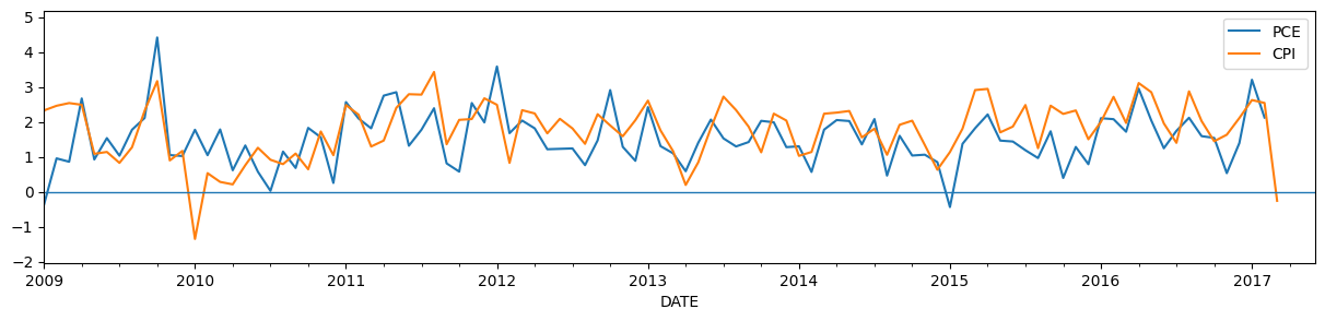
我們選擇這個特定的範例,是因為在 2017 年 3 月,核心 CPI 價格自 2010 年以來首次下跌,而此資訊可能有助於預測該月份的核心 PCE 價格。下圖顯示了在 4 月 14 日觀察到的 CPI 和 PCE 價格數據\(^\dagger\)。
\(\dagger\) 這個說法並不完全正確,因為 CPI 和 PCE 物價指數在事後都可以在一定程度上進行修正。因此,我們提取的序列與 2017 年 4 月 14 日觀察到的序列不完全相同。可以通過從 ALFRED 而不是 FRED 中提取歸檔資料來修正此問題,但我們擁有的數據對於本教學來說已足夠。
[17]:
# Plot the updated dataset
fig, ax = plt.subplots(figsize=(15, 3))
y_post.plot(ax=ax)
ax.hlines(0, '2009', '2017-06', linewidth=1.0)
ax.set_xlim('2009', '2017-06');
為了執行此練習,我們首先建立並擬合 DynamicFactor 模型。具體來說:
我們使用單一動態因子(
k_factors=1)我們使用 AR(6) 模型(
factor_order=6)對因子的動態進行建模我們已將一個全為 1 的向量作為外生變數納入(
exog=const_pre),因為我們使用的通膨序列並非平均值為零。
[18]:
mod_pre = sm.tsa.DynamicFactor(y_pre, exog=const_pre, k_factors=1, factor_order=6)
res_pre = mod_pre.fit()
print(res_pre.summary())
This problem is unconstrained.
RUNNING THE L-BFGS-B CODE

           * * *

Machine precision = 2.220D-16
 N =           12     M =           10

At X0         0 variables are exactly at the bounds

At iterate    0    f=  4.81947D+00    |proj g|=  3.24664D-01

At iterate    5    f=  4.62090D+00    |proj g|=  3.53739D-01

At iterate   10    f=  2.79040D+00    |proj g|=  3.87962D-01

At iterate   15    f=  2.54688D+00    |proj g|=  1.35633D-01

At iterate   20    f=  2.45463D+00    |proj g|=  1.04853D-01

At iterate   25    f=  2.42572D+00    |proj g|=  4.92521D-02

At iterate   30    f=  2.42118D+00    |proj g|=  2.82902D-02

At iterate   35    f=  2.42077D+00    |proj g|=  6.08268D-03

At iterate   40    f=  2.42076D+00    |proj g|=  1.04046D-04

           * * *

Tit   = total number of iterations
Tnf   = total number of function evaluations
Tnint = total number of segments explored during Cauchy searches
Skip  = number of BFGS updates skipped
Nact  = number of active bounds at final generalized Cauchy point
Projg = norm of the final projected gradient
F     = final function value

           * * *

   N    Tit     Tnf  Tnint  Skip  Nact     Projg        F
   12     43     66      1     0     0   3.456D-05   2.421D+00
  F =   2.4207581817590249

CONVERGENCE: REL_REDUCTION_OF_F_<=_FACTR*EPSMCH
                                   Statespace Model Results
=============================================================================================
Dep. Variable:                        ['PCE', 'CPI']   No. Observations:                  216
Model:             DynamicFactor(factors=1, order=6)   Log Likelihood                -522.884
                                      + 1 regressors   AIC                           1069.768
Date:                               Thu, 03 Oct 2024   BIC                           1110.271
Time:                                       15:48:15   HQIC                          1086.131
Sample:                                   02-28-1999
                                        - 01-31-2017
Covariance Type:                                 opg
===================================================================================
Ljung-Box (L1) (Q):             4.50, 0.54   Jarque-Bera (JB):         13.09, 12.63
Prob(Q):                        0.03, 0.46   Prob(JB):                   0.00, 0.00
Heteroskedasticity (H):         0.56, 0.44   Skew:                      0.18, -0.16
Prob(H) (two-sided):            0.02, 0.00   Kurtosis:                   4.15, 4.14
                           Results for equation PCE
==============================================================================
                 coef    std err          z      P>|z|      [0.025      0.975]
------------------------------------------------------------------------------
loading.f1     0.5499      0.061      9.037      0.000       0.431       0.669
beta.const     1.7039      0.095     17.959      0.000       1.518       1.890
                           Results for equation CPI
==============================================================================
                 coef    std err          z      P>|z|      [0.025      0.975]
------------------------------------------------------------------------------
loading.f1     0.9033      0.102      8.875      0.000       0.704       1.103
beta.const     1.9621      0.137     14.357      0.000       1.694       2.230
                        Results for factor equation f1
==============================================================================
                 coef    std err          z      P>|z|      [0.025      0.975]
------------------------------------------------------------------------------
L1.f1          0.1246      0.069      1.805      0.071      -0.011       0.260
L2.f1          0.1823      0.072      2.548      0.011       0.042       0.323
L3.f1          0.0178      0.073      0.244      0.807      -0.125       0.160
L4.f1         -0.0700      0.078     -0.893      0.372      -0.224       0.084
L5.f1          0.1561      0.068      2.308      0.021       0.024       0.289
L6.f1          0.1376      0.075      1.842      0.066      -0.009       0.284
                           Error covariance matrix
==============================================================================
                 coef    std err          z      P>|z|      [0.025      0.975]
------------------------------------------------------------------------------
sigma2.PCE     0.5422      0.065      8.287      0.000       0.414       0.670
sigma2.CPI  1.322e-12      0.144   9.15e-12      1.000      -0.283       0.283
==============================================================================

Warnings:
[1] Covariance matrix calculated using the outer product of gradients (complex-step).
有了擬合模型後,我們現在建構觀察到 2017 年 3 月 CPI 相關的新聞和影響。更新後的資料是 2017 年 2 月和 2017 年 3 月的一部分,我們將檢視對 3 月和 4 月的影響。
在單變數範例中,我們首先建立一個更新後的結果物件,然後將其傳遞給 news 方法。在這裡,我們直接傳遞更新後的資料集來建立新聞。
請注意
y_post包含整個更新後的資料集(而不僅僅是新的資料點)我們還必須傳遞一個更新後的
exog陣列。此陣列必須涵蓋兩者與
y_post相關的整個期間在
y_post結束後,直到由end指定的最後影響日期的任何額外資料點
在此,
y_post在 2017 年 3 月結束,因此我們需要將我們的exog延伸到下一個期間,即 2017 年 4 月。
[19]:
# Create the news results
# Note
const_post_plus1 = np.ones(len(y_post) + 1)
news = res_pre.news(y_post, exog=const_post_plus1, start='2017-03', end='2017-04')
注意:
在上面的單變數範例中,我們首先建構一個新的結果物件,然後將其傳遞給
news方法。我們也可以在這裡這樣做,儘管需要一個額外的步驟。由於我們要求對y_post結束後的期間產生影響,我們仍然需要在該期間將exog變數的額外值傳遞給newsres_post = res_pre.apply(y_post, exog=const_post) news = res_pre.news(res_post, exog=[1.], start='2017-03', end='2017-04')
現在我們已經計算出 news,列印 summary 是檢視結果的便捷方式。
[20]:
# Show the summary of the news results
print(news.summary())
                                      News
===============================================================================
Model:                  DynamicFactor   Original sample:                1999-02
Date:                Thu, 03 Oct 2024                                 - 2017-01
Time:                        15:48:16   Update through:                 2017-03
                                        # of revisions:                       0
                                        # of new datapoints:                  3
                                  Impacts
===========================================================================
impact date impacted variable estimate (prev) impact of news estimate (new)
---------------------------------------------------------------------------
    2017-03               CPI            2.07          -2.33          -0.26
        NaT               PCE            1.77          -1.42           0.35
    2017-04               CPI            1.90          -0.23           1.67
        NaT               PCE            1.67          -0.14           1.53
                  News from updated observations:
===================================================================
update date updated variable   observed forecast (prev)        news
-------------------------------------------------------------------
    2017-02              CPI       2.54            2.24        0.30
                         PCE       2.12            1.87        0.25
    2017-03              CPI      -0.26            2.07       -2.33
===================================================================
/opt/hostedtoolcache/Python/3.10.15/x64/lib/python3.10/site-packages/statsmodels/tsa/statespace/news.py:936: FutureWarning: Setting an item of incompatible dtype is deprecated and will raise in a future error of pandas. Value '0    2.07
1    1.77
2    1.90
3    1.67
Name: estimate (prev), dtype: object' has dtype incompatible with float64, please explicitly cast to a compatible dtype first.
  impacts.iloc[:, 2:] = impacts.iloc[:, 2:].map(
/opt/hostedtoolcache/Python/3.10.15/x64/lib/python3.10/site-packages/statsmodels/tsa/statespace/news.py:936: FutureWarning: Setting an item of incompatible dtype is deprecated and will raise in a future error of pandas. Value '0    0.00
1    0.00
2    0.00
3    0.00
Name: impact of revisions, dtype: object' has dtype incompatible with float64, please explicitly cast to a compatible dtype first.
  impacts.iloc[:, 2:] = impacts.iloc[:, 2:].map(
/opt/hostedtoolcache/Python/3.10.15/x64/lib/python3.10/site-packages/statsmodels/tsa/statespace/news.py:936: FutureWarning: Setting an item of incompatible dtype is deprecated and will raise in a future error of pandas. Value '0    -2.33
1    -1.42
2    -0.23
3    -0.14
Name: impact of news, dtype: object' has dtype incompatible with float64, please explicitly cast to a compatible dtype first.
  impacts.iloc[:, 2:] = impacts.iloc[:, 2:].map(
/opt/hostedtoolcache/Python/3.10.15/x64/lib/python3.10/site-packages/statsmodels/tsa/statespace/news.py:936: FutureWarning: Setting an item of incompatible dtype is deprecated and will raise in a future error of pandas. Value '0    -2.33
1    -1.42
2    -0.23
3    -0.14
Name: total impact, dtype: object' has dtype incompatible with float64, please explicitly cast to a compatible dtype first.
  impacts.iloc[:, 2:] = impacts.iloc[:, 2:].map(
/opt/hostedtoolcache/Python/3.10.15/x64/lib/python3.10/site-packages/statsmodels/tsa/statespace/news.py:936: FutureWarning: Setting an item of incompatible dtype is deprecated and will raise in a future error of pandas. Value '0    -0.26
1     0.35
2     1.67
3     1.53
Name: estimate (new), dtype: object' has dtype incompatible with float64, please explicitly cast to a compatible dtype first.
  impacts.iloc[:, 2:] = impacts.iloc[:, 2:].map(
/opt/hostedtoolcache/Python/3.10.15/x64/lib/python3.10/site-packages/statsmodels/tsa/statespace/news.py:1328: FutureWarning: Setting an item of incompatible dtype is deprecated and will raise in a future error of pandas. Value '0     2.54
1     2.12
2    -0.26
Name: observed, dtype: object' has dtype incompatible with float64, please explicitly cast to a compatible dtype first.
  data.iloc[:, 2:] = data.iloc[:, 2:].map(
/opt/hostedtoolcache/Python/3.10.15/x64/lib/python3.10/site-packages/statsmodels/tsa/statespace/news.py:1328: FutureWarning: Setting an item of incompatible dtype is deprecated and will raise in a future error of pandas. Value '0    2.24
1    1.87
2    2.07
Name: forecast (prev), dtype: object' has dtype incompatible with float64, please explicitly cast to a compatible dtype first.
  data.iloc[:, 2:] = data.iloc[:, 2:].map(
/opt/hostedtoolcache/Python/3.10.15/x64/lib/python3.10/site-packages/statsmodels/tsa/statespace/news.py:1328: FutureWarning: Setting an item of incompatible dtype is deprecated and will raise in a future error of pandas. Value '0     0.30
1     0.25
2    -2.33
Name: news, dtype: object' has dtype incompatible with float64, please explicitly cast to a compatible dtype first.
  data.iloc[:, 2:] = data.iloc[:, 2:].map(
由於我們有多個變數,因此預設情況下,摘要僅顯示來自更新資料以及總影響的新聞。
從第一個表格中,我們可以看到我們更新後的資料集包含三個新的資料點,這些資料的大部分「新聞」來自 2017 年 3 月的非常低的讀數。
第二個表格顯示,這三個資料點大幅影響了對 2017 年 3 月 PCE 的估計(尚未觀察到)。此估計值向下修正了近 1.5 個百分點。
更新後的資料也影響了第一個樣本外月份(即 2017 年 4 月)的預測。納入新資料後,該模型對該月份 CPI 和 PCE 通膨的預測分別向下修正了 0.29 和 0.17 個百分點。
雖然這些表格顯示了「新聞」和總影響,但它們並未顯示每個影響中有多少是由每個更新的資料點造成的。要查看該資訊,我們需要查看詳細資料表格。
查看詳細資料表格的一種方法是將 include_details=True 傳遞給 summary 方法。但是,為了避免重複上面的表格,我們將直接呼叫 summary_details 方法。
[21]:
print(news.summary_details())
                             Details of news for [updated variable = CPI]
======================================================================================================
update date   observed forecast (prev) impact date impacted variable        news     weight     impact
------------------------------------------------------------------------------------------------------
    2017-02       2.54            2.24     2017-04               CPI        0.30       0.18       0.06
                                                                 PCE        0.30       0.11       0.03
    2017-03      -0.26            2.07     2017-03               CPI       -2.33        1.0      -2.33
                                                                 PCE       -2.33       0.61      -1.42
                                           2017-04               CPI       -2.33       0.12      -0.29
                                                                 PCE       -2.33       0.08      -0.18
======================================================================================================
此表格顯示,上述對 2017 年 4 月 PCE 估計值的修正主要來自 2017 年 3 月發布 CPI 相關的新聞。相比之下,2 月發布的 CPI 對 4 月的預測只有一點點影響,而 2 月發布的 PCE 則幾乎沒有影響。
參考文獻
Bańbura, Marta, Domenico Giannone, 和 Lucrezia Reichlin. “Nowcasting.” The Oxford Handbook of Economic Forecasting. 2011 年 7 月 8 日。
Bańbura, Marta, Domenico Giannone, Michele Modugno, 和 Lucrezia Reichlin. “Now-casting and the real-time data flow.” In Handbook of economic forecasting, vol. 2, pp. 195-237. Elsevier, 2013.
Bańbura, Marta, 和 Michele Modugno. “Maximum likelihood estimation of factor models on datasets with arbitrary pattern of missing data.” Journal of Applied Econometrics 29, no. 1 (2014): 133-160.
Knotek, Edward S., 和 Saeed Zaman. “Nowcasting US headline and core inflation.” Journal of Money, Credit and Banking 49, no. 5 (2017): 931-968.